
Code
# Use this R-Chunk to load all your libraries!

# run this line once in the console to get package
# if (!requireNamespace("data4led", quietly = TRUE)) remotes::install_github("byuidatascience/data4led")
library(data4led)This project outline and background information have been provided to assist you as you complete your project. You should assume the reader of your work has no knowledge or access to this information.
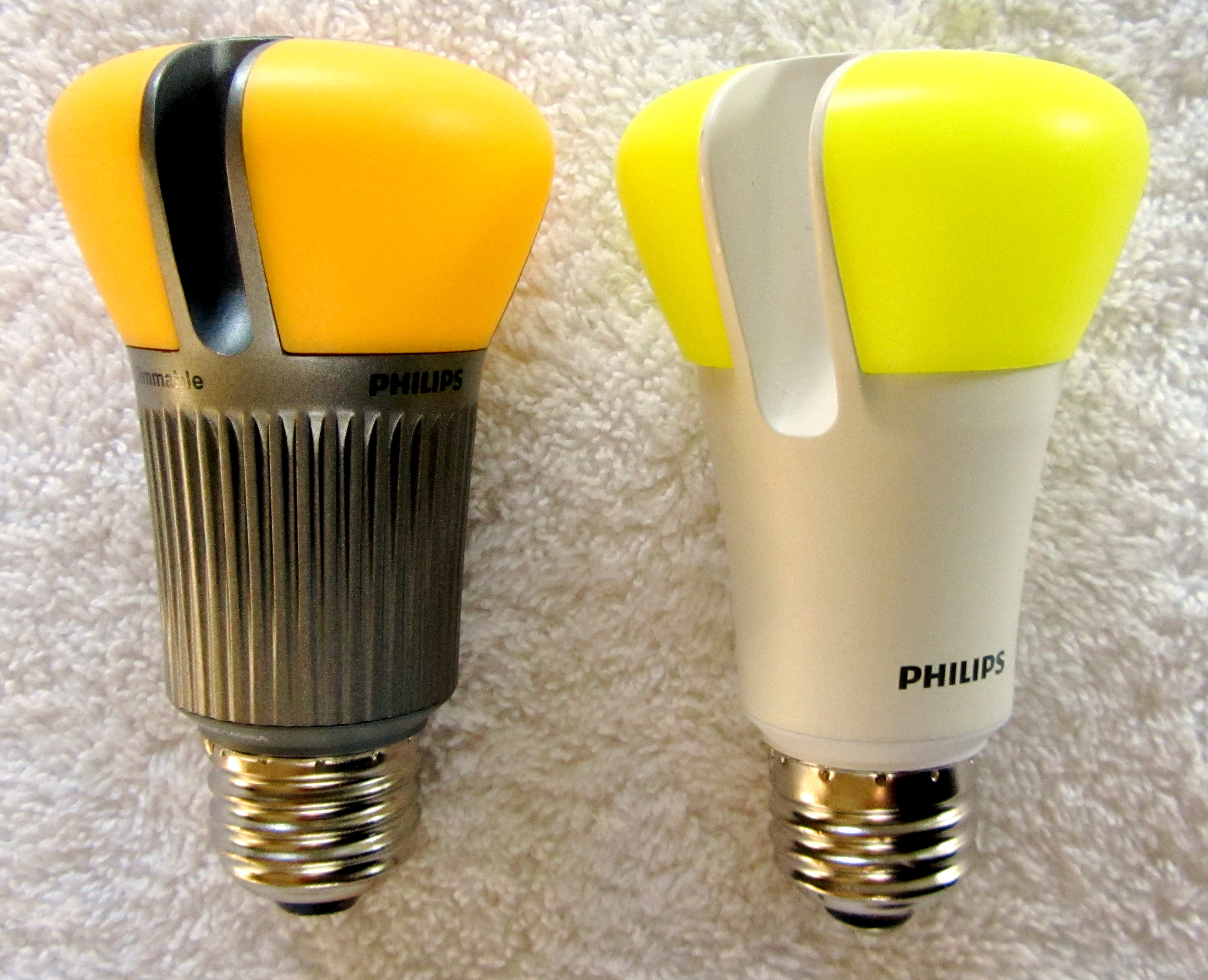
How long does an LED light bulb last? The US Department of Energy launched the Bright Tomorrow Lighting Prize (or L Prize) in 2008 to “spur lighting manufacturers to develop high-quality, high-efficiency solid-state lighting products to replace the common incandescent light bulb.” In addition to requiring less than 10 watts, the winning bulb needed to have a lifetime longer than 25,000 hours. For this project, we will use 80% of the initial intensity1 as the threshold for determining the lifetime of a light bulb.
Phillips won the prize in 2011, after undergoing 18 months of rigorous testing. Note however that there are only 8760 hours in a year (24 hours a day for 365 days), which means 18 months of testing is only 13,140 hours much less than the 25,000 hours required to win the prize. And the data we are using, not the Phillips data, only has measurement for 5010 hours. How do we know the bulb met the requirements to win with only 18 months (or in our case only about 208 days) of testing? We use mathematical models.
When you first turn on an LED bulb, the lumen output slightly increases for a while, going above 100% of the initial brightness. After peaking above 100%,the lumen output stays relatively constant before it starts a slow decent downwards.
In this project, we’ll be fitting the data to deterministic models by maximizing the loglikelihood of the errors. Each of the deterministic models are functions \(f(t)\) that describe the average behavior of lumen output of LED bulbs (as a percent of the initial lumens) after \(t\) hours.
embed-resources: true so your rendered .html inlines all plots — required so the file you upload to Canvas displays your charts. See Quarto Hints for a working YAML template.seed= argument in the led_bulb() function to set the seed and use the following code to read in the light bulb data.# Use this R-Chunk to load all your libraries!
# run this line once in the console to get package
# if (!requireNamespace("data4led", quietly = TRUE)) remotes::install_github("byuidatascience/data4led")
library(data4led)# Use this R-Chunk to import all your datasets!
# Enter the seed as your birthday MMDD.
# bulb <- led_bulb(1, seed = MMDD)This code creates a data frame called “bulb”. The bulb data frame contains measurements for one randomly selected bulb at many time points. You will need to set the seed so that you will have your own random, but reproducible, data with which to work. Please set the seed as the four digit number corresponding to your birthday month and date, MMDD.
head(bulb) to view the first 6 lines of the bulb data frame. Verify that it includes the columns
Beneath the instructions for this task, two sections titled “Maximum Likelihood Method for \(f_2\)” and “Maximum Likelihood Method for \(f_6\)” each apply the maximum likelihood method to the functions \(f_2\) and \(f_6\), using the random seed 123. Read each section, then adapt the code to work with your assigned random seed.
Consider the model \(f_2(t; a_1, a_2) = 100 + a_1t + a_2t^2\). The function \(f_2\) models the brightness of a lightbulb, measured as a percent of the original intensity of the lightbulb, given the number of hours the lightbulb has been on, \(t\). We will fit \(f_2\) to the list of 44 measurements, \((t_i, y_i)\), obtained from the data4led package using the seed 123.
Assuming the residuals (or errors) are independent and normally distributed (with mean 0 and standard deviation 1), the loglikelihood function for these errors is \[\ell_2(a_1,a_2; \mathbf{t},\mathbf{y}) = 44\ln\left(\frac{1}{\sqrt{2\pi}}\right) + \sum_{i=1}^{44} \left(-\frac{1}{2}(y_i - 100 - a_1t_i - a_2t_i^2)^2\right).\] We want to find the maximum of \(\ell_2\). The first partials of \(\ell_2\) are
To find the critical points of \(\ell_2\), we set each partial derivative above equal to zero and then solve \[\left\{ \begin{array}{ll} \left(\sum_{i=1}^{44} (y_i - 100)t_i\right) - \left(\sum_{i=1}^{44}t_i^2\right)a_1 - \left(\sum_{i=1}^{44}t_i^3\right)a_2 &= 0 \\ \left(\sum_{i=1}^{44} (y_i - 100)t_i^2\right) - \left(\sum_{i=1}^{44}t_i^3\right)a_1 - \left(\sum_{i=1}^{44}t_i^4\right)a_2 &= 0. \end{array} \right.\] This system is of the form \[\left\{ \begin{aligned} b_1 - c_{11}a_1 - c_{12}a_2 &= 0 \\ b_2 - c_{21}a_1 - c_{22}a_2 &= 0, \end{aligned} \right.\] with \(c_{11} = \sum t_i^2\), \(c_{12} = c_{21} = \sum t_i^3\), \(c_{22} = \sum t_i^4\), \(b_1 = \sum (y_i - 100)t_i\), and \(b_2 = \sum (y_i - 100)t_i^2\). Each is just a constant that depends on the given data; we calculate (and store) their values using the R code below.
library(data4led)
bulb <- led_bulb(1, seed = 123)  # Remember to use your assigned seed!

t <- bulb$hours
y <- bulb$percent_intensity

c11 <- sum(t^2)
c12 <- sum(t^3)
c22 <- sum(t^4)
b1  <- sum((y - 100) * t)
b2  <- sum((y - 100) * t^2)
The solution to this system is \(a_2 = \frac{c_{11}b_2 - c_{12}b_1}{c_{11}c_{22} - c_{12}^2}\) and \(a_1 = \frac{b_1 - c_{12}a_2}{c_{11}}\).
best_a2 <- (c11 * b2 - c12 * b1) / (c11 * c22 - c12^2)
best_a1 <- (b1 - c12 * best_a2) / c11
best_a1
[1] 0.001190918best_a2[1] -1.743522e-07The critical point for \(\ell_2\) is \((a_1, a_2) = (0.0011909, -1.7435215\times 10^{-7})\). The second partials are \(\frac{\partial^2\ell_2}{\partial a_1^2} = -\sum t_i^2\), \(\frac{\partial^2\ell_2}{\partial a_2^2} = -\sum t_i^4\), and \(\frac{\partial^2\ell_2}{\partial a_2 \partial a_1} = -\sum t_i^3\). The second derivative test uses \(D = \left(\frac{\partial^2\ell_2}{\partial a_1^2}\right)\left(\frac{\partial^2\ell_2}{\partial a_2^2}\right) - \left(\frac{\partial^2\ell_2}{\partial a_2 \partial a_1}\right)^2\).
D <- (-c11) * (-c22) - (-c12)^2
D
[1] 1.23003e+23-c11[1] -328767530Since \(D > 0\) and \(\frac{\partial^2\ell_2}{\partial a_1^2} < 0\), the critical point is a local maximum. Our best fit model is \(f_2(t) = 100 + (0.0011909)t + (-1.7435215\times 10^{-7})t^2\) where \(t \geq 0\).
f2 <- function(x, a1 = best_a1, a2 = best_a2) {
  100 + a1 * x + a2 * x^2
}

x <- seq(-10, 80001, 2)
par(mfrow = c(1, 2), mar = c(2.5, 2.5, 1, 0.25))
plot(t, y, xlab = "Hour", ylab = "Intensity(%)", pch = 16, main = "f2")
lines(x, f2(x), col = 2)
plot(t, y, xlab = "Hour", ylab = "Intensity(%)", pch = 16,
     xlim = c(-10, 80000), ylim = c(-10, 120))
lines(x, f2(x), col = 2)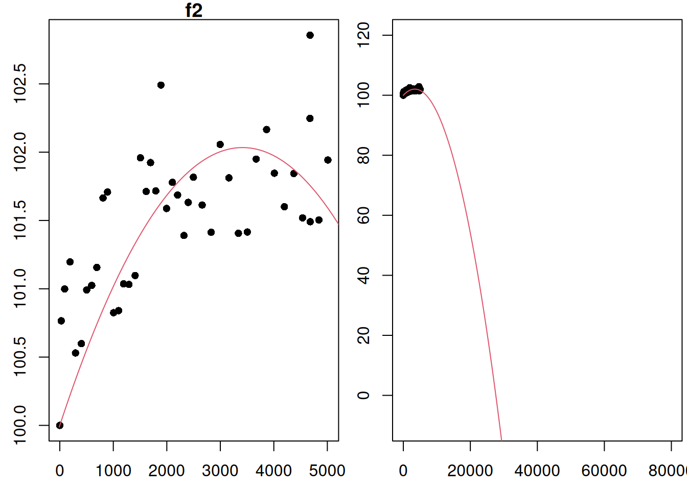
The fitted function provides a good visual fit. The story told by this model suggests that the light bulb will burn out (hit 80% intensity) somewhere between 10 and 20 thousand hours.
Consider \(f_6(t; a_1, a_2) = 100 + a_1t + a_2(1 - e^{-0.0003t})\). The loglikelihood function is \[\ell_6(a_1,a_2; \mathbf{t},\mathbf{y}) = 44\ln\left(\frac{1}{\sqrt{2\pi}}\right) - \frac{1}{2}\sum_{i=1}^{44} (y_i - 100 - a_1t_i - a_2(1 - e^{-0.0003t_i}))^2.\] We apply the maximum likelihood method using the data from our seed.
bulb <- led_bulb(1, seed = 123)  # Remember to use your assigned seed!

t <- bulb$hours
y <- bulb$percent_intensity
Setting each partial derivative to zero gives a system of the form \(b_1 - c_{11}a_1 - c_{12}a_2 = 0\) and \(b_2 - c_{21}a_1 - c_{22}a_2 = 0\), where \(c_{11} = \sum t_i^2\), \(c_{12} = \sum t_i(1 - e^{-0.0003t_i})\), \(c_{22} = \sum (1 - e^{-0.0003t_i})^2\), \(b_1 = \sum (y_i - 100)t_i\), and \(b_2 = \sum (y_i - 100)(1 - e^{-0.0003t_i})\).
c11 <- sum(t^2)
c12 <- sum(t * (1 - exp(-0.0003 * t)))
c22 <- sum((1 - exp(-0.0003 * t))^2)
b1  <- sum((y - 100) * t)
b2  <- sum((y - 100) * (1 - exp(-0.0003 * t)))

best_a2 <- (c11 * b2 - c12 * b1) / (c11 * c22 - c12^2)
best_a1 <- (b1 - c12 * best_a2) / c11
best_a1
[1] -0.0008219878best_a2[1] 7.442637The second partials are \(\frac{\partial^2 \ell_6}{\partial a_1^2} = -\sum t_i^2\), \(\frac{\partial^2 \ell_6}{\partial a_2^2} = -\sum (1 - e^{-0.0003t_i})^2\), and \(\frac{\partial^2\ell_6}{\partial a_2 \partial a_1} = -\sum t_i(1 - e^{-0.0003t_i})\).
D <- (-c11) * (-c22) - (-c12)^2
D
[1] 73001831-c11[1] -328767530Since \(D > 0\) and \(\frac{\partial^2\ell_6}{\partial a_1^2} < 0\), the critical point is a local maximum. Our best fit model is \(f_6(t) = 100 + (-8.2198784\times 10^{-4})t + (7.4426368)(1 - e^{-0.0003t})\) where \(t \geq 0\).
f6 <- function(x, a1 = best_a1, a2 = best_a2) {
  100 + a1 * x + a2 * (1 - exp(-0.0003 * x))
}

x <- seq(-10, 80001, 2)
par(mfrow = c(1, 2), mar = c(2.5, 2.5, 1, 0.25))
plot(t, y, xlab = "Hour", ylab = "Intensity(%)", pch = 16, main = "f6")
lines(x, f6(x), col = 2)
plot(t, y, xlab = "Hour", ylab = "Intensity(%)", pch = 16,
     xlim = c(-10, 80000), ylim = c(-10, 120))
lines(x, f6(x), col = 2)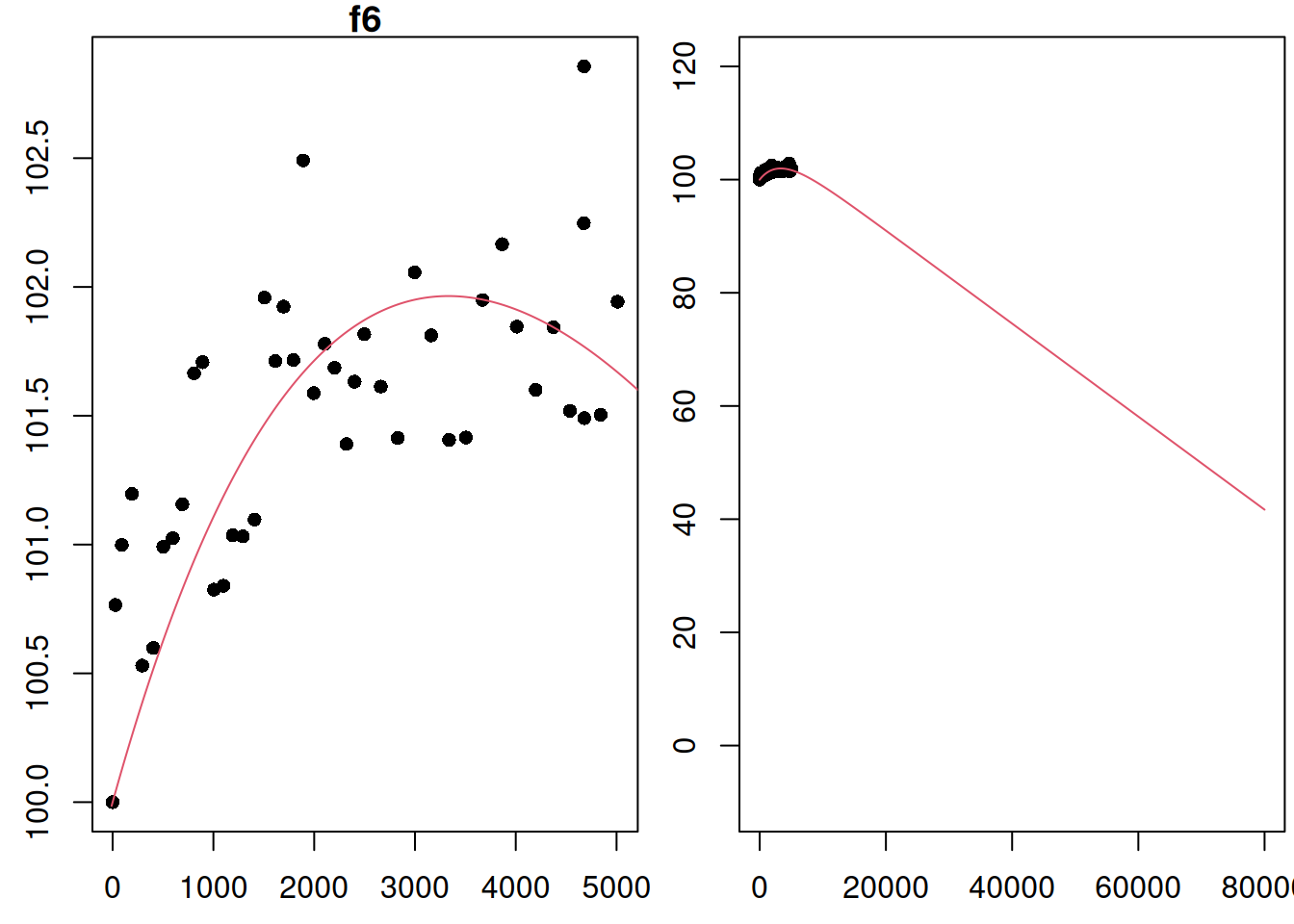
The fitted function provides a good visual fit. The light bulb will burn out (hit 80% intensity) somewhere around 30,000 hours.
Create a new Quarto document.
Answer the question, “How long does an LED light bulb last?”
uniroot() function in R to find the approximate solution for where each of your five fitted models is at 80% of the initial intensity, solve the equation \(f_i(t) = 80\) for each of the five fitted models.
Organize your work into a cohesive analysis and submit it to Canvas. Your narrative should stand alone apart from the “project instructions” (meaning your reader should not need the instructions for the project to understand what you are doing or explaining) and separate from the individual Tasks (meaning you should not assume your reader has read any of your previous narratives). It is your job in the narrative to lead your reader from the background and question to given data and 5 general models, fitting those models, and answering a question about the data using those fitted models.
Reflect on your work for this project. At the bottom of your report include the following in a brief (1-2 paragraph) reflection.
This number is a simplified story for illustrative purposes only.↩︎