Class 15

Between Class Sessions - Prep for Day 15

Please spend around 2 hours working between class sessions, focusing on the tasks below. Use any extra time to complete KnewtonAlta assignments and/or work on Project tasks.

Pick something from your prep today that you can share with your group in class. It might be something new that you learned. It might be questions you have that are still unanswered, or a question along with what helped you eventually answer it. It might be something tricky that you solved. It might be a review topic that helped you remember something. It might be a conversation you had with AI that was helpful. You will have a chance to share this with your peers during class. Come ready to articulate your thinking and questions.

Preparation

(1) Likelihood Practice (with Poisson)

Use the storms listed on Wikipedia’s List of Florida hurricanes page to answer the questions below.

1. Use the data from 2005-2007 for \(x_1\), \(x_2\), and \(x_3\). The number of storms in 2005 is \(x_1\), the number of storms in 2006 is \(x_2\), and the number of storms in 2007 is \(x_3\).

• Adapt the code from class to complete the following table, calculating the probability given the value of \(\lambda\).

p3v1 <- function(x,lambda=2){
# each element of x must be a whole number
  prod((lambda^x/factorial(x))*exp(-lambda))
}

p3v1(c(8,2,8),1)
p3v1(c(8,2,8),2)

\(\lambda\)	\(P(X_1=x_1,X_2=x_2,X_3=x_3)\)
1	1.531x\(10^{-11}\)
2	1.998x\(10^{-7}\)
3
4
5
6
7
8
9
10
11
12
13
14
15

• Use the code below to plot this function of \(\lambda\) in R. (Because both \(\lambda\) and \(x\) are vectors, we must use the sapply function from R to appropriately tell the computer how to to parse the notation. You do not have to modify any code involving sapply for future tasks, so feel free to just run the code below to produce the needed plot.)

lambda <- seq(0,15,0.01)
x <- c(8,2,8)
probs <- sapply(lambda, p3v1, x = x)
plot(lambda, probs, type='l')

• If we know there will be 8 Florida tropical storms this year, 2 Florida tropical storms next year, and 8 Florida tropical storms the year after that (in other words the data values from 2005-2007), what is your guess for the best choice of parameter \(\lambda\)?

2. Using the data from 2010-2012 adapt the code from exercise 1 (above) to plot a function with \(\lambda\) on the horizontal axis and probability (that of the number of storms this year will be the same as the number of storms in 2010, the number of storms next year will be the same as the number of storms in 2011, and the number of storms in the year after that will be the same number as the number of storms in 2012) on the vertical axis. See Wikipedia’s List of Florida hurricanes to get the appropriate data.

• Using your plot what is your guess for the best choice of the parameter \(\lambda\) in this case?

3. Using the data from 2012-2015 adapt the code to plot a function with \(\lambda\) on the horizontal axis and probability (that of the number of storms this year will be the same as the number of storms in 2012, the number of storms next year will be the same as the number of storms in 2013, the number of storms in the year after that will be the same number as the number of storms in 2014, and the number of storms in the year after that will be the same number as the number of storms in 2015) on the vertical axis.

• Note: There are 4 years this time. How will you have to change the code to allow for this?
• Using your plot what is your guess for the best choice of the parameter \(\lambda\) in this case?

4. Using the data from 2000 and 2001 adapt the code to plot a function with \(\lambda\) on the horizontal axis and probability on the vertical axis.

• Note: There are 2 years this time. How will you have to change the code to allow for this?
• Using your plot what is your guess for the best choice of the parameter \(\lambda\) in this case?

5. Using the data from 2019 and 2020 adapt the code to plot a function with \(\lambda\) on the horizontal axis and probability on the vertical axis.

• Note: There are 2 years this time. How will you have to change the code to allow for this?
• Using your plot what is your guess for the best choice of the parameter \(\lambda\) in this case?

(2) Residuals Exercises

Residuals

The residual for an observation is defined as the vertical distance between the observed value, \(y\), and value predicted by a fitted model, represented with a \(\hat{y}\) (read “y hat”).

Examples:

Given the model \(f(x) = ax^2 + bx + c\) and the data point \((x, y)\), the residual is

\[ \begin{aligned} y - \hat{y} &= y - f(x) \\ &= y - (ax^2 + bx + c) \\ &= y - ax^2 - bx - c \end{aligned} \]

Given the model \(g(x) = k\) and the data point \((x, y)\), the residual is

\[ \begin{aligned} y - \hat{y} &= y - g(x) \\ &= y - k \end{aligned} \]

Given the model \(h(x) = ae^{-bx} + cxe^{-bx}\) and the data point \((x, y)\), the residual is

\[ \begin{aligned} y - \hat{y} &= y - h(x) \\ &= y - (ae^{-bx} + cxe^{-bx}) \\ &= y - ae^{-bx} - cxe^{-bx} \end{aligned} \]

Consider the 6 functions you have been fitting in Project 1.

• Write down a formula for the residual given model \(f_1\)
• Write down a formula for the residual given model \(f_2\)
• Write down a formula for the residual given model \(f_3\)

Regular Reminders

Applied Practice (Project Work)

• Complete Project 1 Task 4

During Class

Brain Gains

• Critique the following visual fits for \(f_5\).

  • 

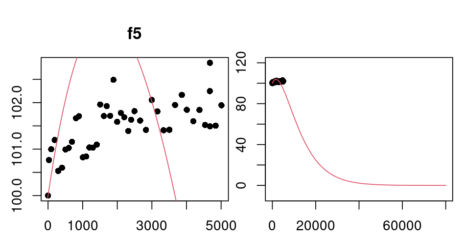
    Visual fit 1 for f5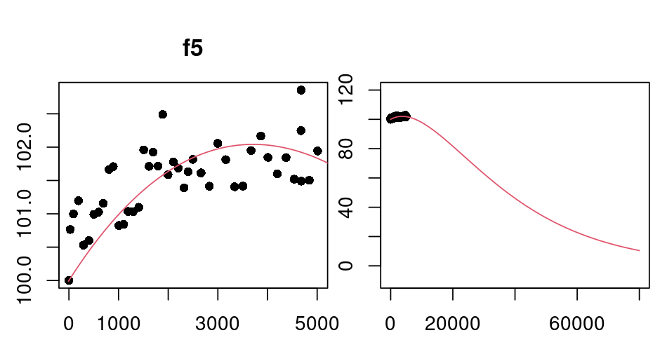

  • 

    Visual fit 2 for f5

• Write down a formula for the residual, \(y - \hat{y}\), given the model \(f(x) = b + mx\) and data point \((x,y) = (4,7)\)
• Write down a formula for the residual, \(y - \hat{y}\), given the model \(g(x) = c + bx + a\ln(4x)\) and data point \((x,y) = (x_3,y_3)\)

Answers

Given the model \(f(x) = b + mx\) and the data point \((x, y) = (4, 7)\), the residual is

\[ \begin{aligned} y - \hat{y} &= y - f(x) \\ &= 7 - (b + m\cdot 4) \\ &= 7 - b - 4m \end{aligned} \]

Given the model \(g(x) = c + bx + a\ln(4x)\) and the data point \((x, y) = (x_3, y_3)\), the residual is

\[ \begin{aligned} y - \hat{y} &= y_3 - g(x_3) \\ &= y_3 - \bigl(c + bx_3 + a\ln(4x_3)\bigr) \\ &= y_3 - c - bx_3 - a\ln(4x_3) \end{aligned} \]

In the formula \(r = y - f(x)\), we just replace \(x\), \(y\), and \(f(x)\) with what they equal. We are computing the error between an observed value \(y\) and predicted value \(f(x)\).

• The number of tropical storms observed in Florida during the years 2019, 2020, and 2021 was 7, 13, and then 3 (see List of Florida hurricanes (2000–present) #2019). In the prep we used the Poisson distribution to compute a probability, for various values of \(\lambda\), of observing some number of tropical storms over a 3 year period. Adapt the code from the prep (see below) to construct a plot of \(\lambda\) versus the probability of seeing 7, 13, and then 3 storms, for that value of \(\lambda\). What is your guess for the best choice of parameter \(\lambda\)?

p3v1 <- function(x,lambda=2){
# each element of x must be a whole number
  prod((lambda^x/factorial(x))*exp(-lambda))
}

lambda <- seq(0,15,0.01)
x <- c(8,2,8) #how many storms
probs <- sapply(lambda, p3v1, x = x)
plot(lambda,probs,type='l')

Discussion

Likelihood

The Poisson distribution is modeled using the function (called a probability mass function)

• \(p(x; \lambda) = \frac{\lambda^x}{x!}e^{-\lambda}\) for every \(x = 0, 1, 2, 3, ...\), for some \(\lambda > 0\).

The likelihood function for the Poisson distribution is the function

• \(L_1(\lambda; x) = \frac{\lambda^x}{x!}e^{-\lambda}\) for every \(\lambda > 0\), for some \(x = 0, 1, 2, 3, ...\).

What do you notice about \(L_1\) and \(p\)? What are the similarities? What are the differences?

• Each value of \(\lambda\) gives a specific probability function \(p\).
• Each value of \(x\) is an observation made. We can plug \(x\) into a specific probability function, to get a probability, or we can use that value of \(x\) to create a specific likelihood function.

---

We created the joint probability mass function for three independent Poisson Random variables by multiplying three functions together to obtain

• \(p_3(x_1, x_2, x_3; \lambda) = \frac{\lambda^{x_1 + x_2 + x_3}}{x_1!x_2!x_3!}e^{-3\lambda}\) for every \(x_1 = 0, 1, 2, 3, ...\), \(x_2 = 0, 1, 2, 3, ...\), and \(x_3 = 0, 1, 2, 3, ...\), for some \(\lambda > 0\).

Consider the function

• \(L_3(\lambda; x_1, x_2, x_3) = \frac{\lambda^{x_1 + x_2 + x_3}}{x_1!x_2!x_3!}e^{-3\lambda}\) for every \(\lambda > 0\), for some \(x_1 = 0, 1, 2, 3, ...\), \(x_2 = 0, 1, 2, 3, ...\), and \(x_3 = 0, 1, 2, 3, ...\).

What do you notice about \(L_3\) and \(p_3\)? What are the similarities? What are the differences?

• Each value of the parameter \(\lambda\) gives a specific probability function \(p_3\).
• Each set of values \(x_1\), \(x_2\), \(x_3\) is a potential outcome from the chance experiment (how many storms). These values can be inserted into a specific probability function to compute a single probability, or they can be used to create a likelihood function.

When calculating probability we use \(p\) (or \(p_3\)) and we assume the parameter selected is trustworthy. We are assuming a specific model and then calculate probabilities using the specific model (we selected and fixed the parameter \(\lambda\)).

When calculating likelihood we use \(L_1\) (or \(L_3\)) and we are trying to determine the trustworthiness of each potential choice for \(\lambda\) given what we have observed (our data). We are fixing the value of \(x\) and considering how trustworthy each value of \(\lambda\) is, given that specific \(x\) we observed.

Likelihood Function

The likelihood function gives the likelihood, or probability (in these examples), of the data as a function of the unknown parameter value(s).

Source: These definitions are taken from OpenStax Introductory Statistics and Modeling the Dynamics of Life by Adler.

We can use the likelihood function to answer the question, “What is the most likely parameter value(s) given the data?” or “Which parameter value(s) should we trust the most given what we have observed?”

Group Meeting

Start by giving each person a moment to share what they chose to prepare for class. Help each other address any questions. When each person has had a chance to share, move on the other activities.

Activity - Residual Practice

Residuals

The residual for an observation is defined as the vertical distance between the observed value, \(y\), and value predicted by a fitted model, represented with a \(\hat{y}\) (read “y hat”).

Examples:

Given the model \(f(x) = ax^2 + bx + c\) and the data point \((x, y)\), the residual is

\[ \begin{aligned} y - \hat{y} &= y - f(x) \\ &= y - (ax^2 + bx + c) \\ &= y - ax^2 - bx - c \end{aligned} \]

Given the model \(g(x) = k\) and the data point \((x, y)\), the residual is

\[ \begin{aligned} y - \hat{y} &= y - g(x) \\ &= y - k \end{aligned} \]

Given the model \(h(x) = ae^{-bx} + cxe^{-bx}\) and the data point \((x, y)\), the residual is

\[ \begin{aligned} y - \hat{y} &= y - h(x) \\ &= y - (ae^{-bx} + cxe^{-bx}) \\ &= y - ae^{-bx} - cxe^{-bx} \end{aligned} \]

• Consider the 6 functions you have been fitting in Project Unit 1.
  • On the chalkboard, write down a formula for the residual given the general model \(f_4\) and data point \((x_i,y_i)\).
  • On the chalkboard, write down a formula for the residual given the general model \(f_5\) and data point \((x_j,y_j)\).

Activity - Likelihood Practice

Use the storms listed on Wikipedia’s List of Florida hurricanes page to answer the questions below. Feel free to head to yesterday’s page to grab code examples to help you work on the things below.

• Using the data from 2005-2009, what is the likelihood that \(\lambda =2\)?
  • Define the likelihood function for this 5 year time period and plot it in R.
• Using the data from 2010-2016, what is the likelihood that \(\lambda =5\)?
  • Define the likelihood function for this 7 year time period and plot it in R.

Work together to develop code in R that will allow you to quickly use any given time period of \(k\) years to construct a graph of the likelihood function for \(k\) Poisson random variables.

Discussion

Likelihood (not just for Poisson Random Variables)

Key Idea: We can use the likelihood function to answer the question, “What is the most likely parameter value(s) given the data?” or “Which parameter value(s) should we trust the most given what we have observed?”

Likelihood is not probability but it is related to probability.

Poisson Distribution

This is a Poisson distribution. (A common probability model.)

• \(p(x; \lambda) = \frac{\lambda^x}{x!}e^{-\lambda}\) for every \(x = 0, 1, 2, 3, ...\), for some \(\lambda > 0\).

If we have more than one observation and we assume the observations come from independent random variables, we can multiply the probability functions to find the joint probability function. This is a probability model, the joint probability mass function for \(n\) Poisson random variables (all with the same \(\lambda\)).

• \(F_P(\mathbf{x}; \lambda) = \prod_{i=1}^n \frac{\lambda^{x_i}}{x_i!}e^{-\lambda}\) for every \(x_i = 0, 1, 2, 3, ...\) with \(i = 1, 2, ... n\), for some \(\lambda > 0\).

How do we go from a distribution to a likelihood function? We reverse the roles of the data (the input variable, or independent variable, a list of measurements) and the parameters. This is the likelihood function for \(n\) Poisson random variables (all with the same \(\lambda\)).

• \(L_P(\lambda; \mathbf{x}) = \prod_{i=1}^n \frac{\lambda^{x_i}}{x_i!}e^{-\lambda}\) for every \(\lambda > 0\), for some \(x_i = 0, 1, 2, 3, ...\) with \(i = 1, 2, ... n\).

We can use the following code to plot this function in R.

Click to view the code.

rm(list=ls())

###Define the distribution###
p <- function(x,lambda=1){
# x must be a whole number
  (lambda^x/factorial(x))*exp(-lambda)
}

###Define the likelihood function###
LP <- function(lambda,x){
# The element of x must be a whole numbers.
  prod(p(x,lambda))
}

###Possible Parameter Values###
lambda <- seq(0,10,0.001)

###Data###
# Florida Hurricane Data (2000-2022)
data <- c(4,4,8,8,6,8,2,8,8,4,8,6,4,3,2,4,6,7,4,7,13,3,3)

#Here we calculate the output from the likelihood function given the observed data.
y <- sapply(lambda,FUN=LP,x=data)

#We plot the likelihood function.
par(mar=c(2.5,2.5,3,0.25))
plot(lambda,y,type='l',main='Poisson Likelihood')

Exponential Distribution

This is an Exponential distribution. (A common probability model.)

• \(f_2(x; \lambda) = \lambda e^{-\lambda x}\) for every \(x > 0\), for some \(\lambda >0\).

When we have more than one observation, and we assume the observations come from independent random variables, then we can multiply the probability functions to find the joint probability function. This is a probability model, the joint probability density function for \(n\) Exponential random variables (all with the same \(\lambda\)).

• \(F_E(\mathbf{x}; \lambda) = \prod_{i=1}^n \lambda e^{-\lambda x_i}\) for every \(x_i > 0\) with \(i = 1, 2, ... n\), for some \(\lambda >0\).

How do we go from a distribution to a likelihood function? Reverse the roles of the data (the input variable, or independent variable, a list of measurements) and the parameters. This is the likelihood function for \(n\) Exponential random variables (all with the same \(\lambda\)).

• \(L_E(\lambda; \mathbf{x}) = \prod_{i=1}^n \lambda e^{-\lambda x_i}\) for every \(\lambda >0\), for some \(x_i > 0\) with \(i = 1, 2, ... n\).

We can use the following code to plot this function in R.

Click to view the code.

###Define the distribution###
f2 <- function(x,lambda=1){
# x and lambda must be positive
  lambda*exp(-lambda*x)
}

###Define the Likelihood function###
LE <- function(lambda,x){
# The elements of x must be positive.
  prod(f2(x,lambda))
}

###Possible Parameter Values###
lambda <- seq(0,10,0.001)

###Data###
# Some Simulated Data (This is data from an Exponential random variable.)
data <- c(0.45729967, 0.47156107, 1.21461705, 0.20539769, 1.78975399, 0.09095850, 0.64675475, 1.60109333, 1.57752679, 0.01238945)

#Here we calculate the output from the likelihood function given the observed data.
y <- sapply(lambda,FUN=LE,x=data)

#We plot the likelihood function.
par(mar=c(2.5,2.5,3,0.25))
plot(lambda,y,type='l',main='Exponential Likelihood')

Normal Distribution

This is a Normal distribution. (A common probability model.)

• \(f_3(x; \mu, \sigma) = \frac{1}{\sqrt{2\pi\sigma^2}}e^{-\frac{(x-\mu)^2}{2\sigma^2}}\) for every real number \(x\), for some real number \(\mu\) and real number \(\sigma > 0\).

If we have more than one observation and we assume the observations come from independent random variables, we can multiply the probability functions to find the joint probability function. This is a probability model, the joint probability density function for \(n\) Normal random variables (all with the same \(\mu\) and \(\sigma\)).

• \(F_N(\mathbf{x}; \mu, \sigma) = \prod_{i=1}^n \frac{1}{\sqrt{2\pi\sigma^2}}e^{-\frac{(x_i-\mu)^2}{2\sigma^2}}\) for every real number \(x_i\) with \(i = 1, 2, ... n\), for some real number \(\mu\) and real number \(\sigma > 0\).

How do we go from a distribution to a likelihood function? Reverse the roles of the data (the input variable, or independent variable, a list of measurements) and the parameters. This is the likelihood function for \(n\) Normal random variables (all with the same \(\mu\) and \(\sigma\)).

• \(L_N(\mu, \sigma; \mathbf{x}) = \prod_{i=1}^n \frac{1}{\sqrt{2\pi\sigma^2}}e^{-\frac{(x_i-\mu)^2}{2\sigma^2}}\) for every real number \(\mu\) and real number \(\sigma > 0\), for some real numbers \(x_i\) with \(i = 1, 2, ... n\).

We can use the following code to plot this function in R.

Click to view the code.

###Define the distribution###
f3 <- function(x,mu=0,s=1){
  (1/sqrt(2*pi*s^2))*exp(-(x-mu)^2/(2*s^2))
}

###Define the likelihood function###
# For simplicity, we'll assume sigma is 1.
LN <- function(mu,sigma=1,x){
  prod(f3(x,mu,sigma))
}

###Possible Parameter Values###
mu <- seq(-10,10,0.001)

###Data###
# Some more Simulated Data (This is data from a Normal random variable.)
data <- c(-3.77117676, -2.91429587, -2.02774901, -0.23984575, -1.41960740, -3.17490528, -3.21755276, -0.06442566, -1.92134953, -0.93160739)

#Here we calculate the output from the likelihood function given the observed data.
y <- sapply(mu,FUN=LN,x=data,sigma=1)

#We plot the likelihood function.
par(mar=c(2.5,2.5,3,0.25))
plot(mu,y,type='l',main='Normal Likelihood')

Deterministic vs Probability Models

Deterministic models describe relationships between quantities.

• time a light bulb is on (quantity 1) and the brightness of the bulb (quantity 2)
• number of months since purchase (quantity 1) and the thickness of a shoe tread (quantity 2)
• number of years (quantity 1) and number of elves (quantity 2)
• distance travel (quantity 2) and wear on vehicle (quantity 2)
• money spent (quantity 1) and money earned (quantity 2)
• time spent studying (quantity 1) and skills learned (quantity 2)
• amount of butter (quantity 1) and chewiness of cookie (quantity 2)

Probability models describe probability information for a measurement.
Measurements have variation. There is always some uncertainty in measurement. Even if we are capable of measuring precisely there can still be variation. For example, we can count with precision how many heads there are in 100 coin flips. But if we repeat the experiment (flipping a coin 100 more times and counting) we could get a different number of heads. If we are measuring the weight of an object, there can be variation in the weights based on precision of the scale and other factors (which scale is used, calibration, temperature, vibrations, user error,…). Because there is variation in measurement we often think of measurements as random (or stochastic) variables and use probability distributions to describe the values and associated probabilities.

• Some Common Probability Models
  • Poisson distribution (discrete)
    • the number of events that occur during a fixed time interval
  • Normal distribution (continuous)
  • Exponential distribution (continuous)
  • Binomial distribution (discrete)
  • Uniform distribution (continuous)
  • Gamma distribution (continuous)

Our focus in Math 119 will be fitting models (extracting information from data and encoding it into parameter values) and using fitted models to answer questions. We will only touch briefly the lowest level of evaluating models (does the story the fitted model tells match already known information).

---

Source: Class.15 on byuimath.com