Class 24

Between Class Sessions - Prep for Day 24

Please spend around 2 hours working between class sessions, focusing on the tasks below. Use any extra time to complete KnewtonAlta assignments and/or work on Project tasks.

Pick something from your prep today that you can share with your group in class. It might be something new that you learned. It might be questions you have that are still unanswered, or a question along with what helped you eventually answer it. It might be something tricky that you solved. It might be a review topic that helped you remember something. It might be a conversation you had with AI that was helpful. You will have a chance to share this with your peers during class. Come ready to articulate your thinking and questions.

Preparation

(1) Writing Equations (more practice)

The goal of these exercises is to practice writing functions that model given situations. Each of the functions you create should depend on only one variable. You’ll need this skill to solve applied optimization problems.

A right circular cone has a volume of 231 cubic inches, which is 1 gallon. (For example, if the height is \(h=5\) inches then the radius is \(r = ?\)). Find a function that gives the radius in terms of its height. What is the domain of this function?
A light-rail system carries 80000 passengers per day at a fare of 2.25 dollars per ride. For each 5-cent increase/decrease in fare, surveys predict ridership will drop/grow by 250 passengers. (For example, if the fare is lowered to 2.00 dollars per ride, then the number of riders is ??? and the revenue is ???). Find a function giving the revenue as a function of \(x\), the number of 5-cent increases. (Hint: first find a formula for the number of riders as a function of \(x\), and the cost per ride as a function of \(x\). Revenue is number of passengers multiplied by the cost per passenger.) What is the domain of this function?

(2) Partial Derivatives of a loglikelihood function

Watch the videos below that walk you through finding the first and second partials of \[ \begin{aligned} \ell_2 &= \ell_2(a_1, a_2;\, \mathbf{t}, \mathbf{y}) \\ &= 44\ln\left(\frac{1}{\sqrt{2\pi}}\right) + \sum_{i=1}^{44} \left(-\frac{1}{2}(y_i - 100 - a_1 t_i - a_2 t_i^2)^2\right). \end{aligned} \]

First Partials (~11 min)
Second Partials (~10 min)
Calculating Constants (~7 min) After watching the videos, try to repeat the computations on your own so that you can discover where you have questions.

Now try repeating these computations yourself for \[\ell_6(a_1,a_2; \mathbf{t},\mathbf{y}) = 44\ln\left(\frac{1}{\sqrt{2\pi}}\right) - \frac{1}{2}\sum_{i}^{44} (y_i - 100 - a_1t_i - a_2(1-e^{-0.0003t}))^2\]

Partial derivatives of loglikelihood for f6.

Click to expand the material used in the videos above.

Applying Partial Derivatives to Loglikelihood

Consider the model \(f_2(t; a_1, a_2) = 100 + a_1t + a_2t^2\). The function \(f_2\) models the brightness of a lightbulb, measured as a percent of the original intensity of the lightbulb, given the number of hours the lightbulb as been on, \(t\). We will fit \(f_2\) to a list of 44 measurements, \((t_i, y_i)\). Assuming the residuals (or errors) are independent and normally distributed (with mean 0 and standard deviation 1), the loglikelihood function for these errors is \(\ell_2(a_1,a_2; \mathbf{t},\mathbf{y}) = 44\ln\left(\frac{1}{\sqrt{2\pi}}\right) + \sum_{i=1}^{44} \left(-\frac{1}{2}(y_i - 100 - a_1t_i - a_2t_i^2)^2\right)\).

Find the first partials of \(\ell_2\).
Find the second partials of \(\ell_2\).

Our data, a list of 44 points \((t_i, y_i)\).

rm(list=ls())
library(data4led)
bulb <- led_bulb(1,seed=0219)

t <- bulb$hours
y <- bulb$percent_intensity

The number \(\sum_{i=1}^{44} t_i(y_i-100)\) is a constant that depends on our data.

A <- sum((y-100)*t)
A

The number \(\sum t_i^2\) is a constant that depends on our data.

B <- sum(t^2)
B

The number \(\sum t_i^3\) is a constant that depends on our data.

C <- sum(t^3)
C

The number \(\sum t_i^2(y_i -100)\) is a constant that depends on our data.

D <- sum((y-100)*t^2)
D

The number \(\sum t_i^4\) is a constant that depends on our data.

E <- sum(t^4)
E

Regular Reminders

Skill Practice (KA Homework)

Complete 2 – Partial Derivatives assignment.

Applied Practice (Project Work)

Start Project 2 Task 2
- Calculate the first derivative of \(\ell_1\) with respect to \(a_1\)
- Calculate the first partial derivatives of \(\ell_4\). Remember there are two first partial derivatives when a function has two independent variables.
- Calculate the first derivative of \(\ell_5\)

During Class

Brain Gains

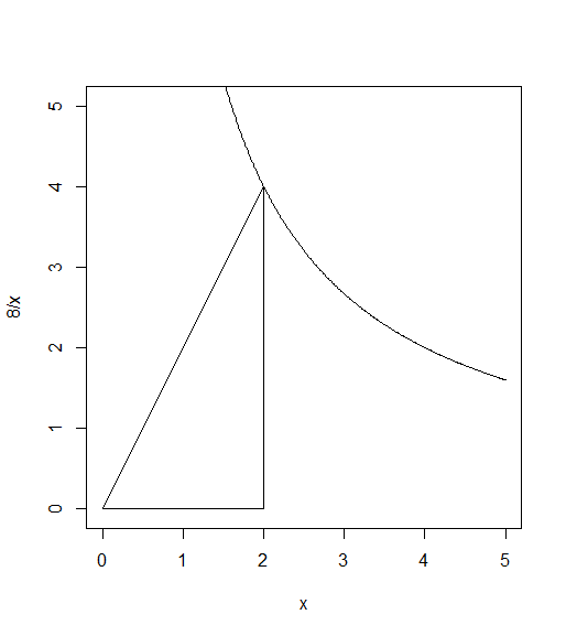
Consider the curve \(y=8/x\) for \(x>0\). Write down a function \(f(x)\) that gives the distance from the origin \((0,0)\) to a point on the curve \(y=8/x\). A plot of the curve is shown below, along with a right triangle that has one vertex at \((0,0)\) and another at a point \((x,8/x)\) on the curve. (Hint: The Pythagorean theorem \(a^2+b^2=c^2\) will help.)

Solution

The Pythagorean theorem here gives \(d^2 = x^2+y^2\). Because \(y=8/x\), we have \(d^2 = x^2+(8/x)^2\). Solving for \(d\) gives the function as \(f(x) = \sqrt{ (x)^2 + (8/x)^2 }\).

Use R to plot the curve \(y=8/x\) as well as the function \(f(x)\) from the previous question. Does \(f(x)\) have a maximum or minimum? Explain.

Solution

We now use R to graph both the equation \(y=8/x\) and the distance function.

f <- function(x){sqrt(x^2 + (8/x)^2)}

#We first plot y = 8/x. Using asp=1 equalizes x and y distances.
x <- seq(0,5, 0.01)
plot(x,8/x, ylim=c(0,5), asp = 1, type = "l")

#Let's add concentric circles to see how far from the origin points are.
symbols(x = rep(0,5), y =rep(0,5), circles = seq(1,5), add = TRUE, inches = FALSE)
#Let's guess x = 3 as the closest spot.  We can see it's a bit to large. 
abline(v=3)

#Now let's plot f and add x=3 for comparison 
plot(x,f(x), ylim=c(0,30), type = "l")
abline(v=3)
#The value x=3 is too large.

#Zoom in. 
x <- seq(2.5,3, 0.01)
plot(x,f(x), ylim=c(3,5), type = "l")
abline(v=2.82)
abline(v=2.84)

#Zoom in. 
x <- seq(2.82, 2.84, 0.001)
plot(x,f(x), ylim=c(3.999,4.001), type = "l")

The plot has a minimum value somewhere a bit less than 3. There has to be a better way to find the minimum than zooming in. This is where derivatives come to the rescue.

Compute the derivative of \(f(x) = \sqrt{x^2+(8/x)^2}\). Then solve \(f'(x) = 0\) using uniroot.

Solution

We first rewrite \(f(x) = \sqrt{x^2+(8/x)^2}\) as \(f(x) = (x^2+64x^{-2})^{1/2}\). The derivative is \(f'(x) = \frac{1}{2}(x^2+64x^{-2})^{-1/2}(2x - 128x^{-3})\). Using uniroot, we obtain \(x = 2.828428\).

f_x <- function(x){1/2*(x^2+64*x^(-2))^(-1/2)*(2*x - 128*x^(-3))}
uniroot(f_x,c(2,3))$root

Discussion

You have been given a list of data for 50 ElvesRUs employees, \((t_i, c_i)\), were \(t_i\) is the number of years working at ElvesRUs and \(c_i\) is the salary for the \(i^{\text{th}}\) employee. The salary (platinum coins per year) for an employee at ElvesRUs can be modeled by \(f(t;A,b,k)=Ae^{bt}+k,\) where \(t\) is the number of years an elf has been working at ElvesRUs. Assume the residuals (errors) are independent and normally distributed (with mean of 0 and standard deviation of 1), which means we’re assuming the probability model for the residuals is \[p(r) = \frac{1}{\sqrt{2\pi}}e^{-\frac{r^2}{2}}\]

Write the loglikelihood function for the errors in this situation.
Rewrite the loglikelihood function using the properties of logs and sums.
Compute the first partial derivatives of the loglikelihood function. (We’ll do one together. The solutions for all three of them are in the file below.) ElvesRUs loglikelihood derivatives (PDF)

Group Meeting

Start by giving each person a moment to share what they chose to prepare for class. Help each other address any questions. When each person has had a chance to share, move on the other activities.

Activity - Loglikelihood Practice, Derivatives, Optimization, and Project 2

You will be working together to revisit Task 1 and complete part of Task 2 for Project 2. The prep for today asked you to watch some videos related to \(f_2\).

Consider the model \(f_1(t; a_1) = 100 + a_1t\).

On the chalk board, as a group, go through the computations needed to obtain the loglikelihood function. Your job is to perform the needed computations and include enough explanations to show that

\[\ell_1(a_1; \mathbf{t},\mathbf{y}) = 44\ln\left(\frac{1}{\sqrt{2\pi}}\right) - \frac{1}{2}\sum_{i}^{44} (y_i - 100 - a_1t_i)^2\]
Compute the first derivative of the loglikelihood function, so compute \(\frac{d\ell_1}{da_1}\). The solution is provided in Task 2.
Now compute the second derivative \(\frac{d^2\ell_1}{da_1^2}\). Again, the solution is provided in Task 2.
Use the following code to plot the loglikelihood function.

rm(list=ls())  #clear the environment
library(data4led) #load the library
#read in the data set, using seed 123 for class comparisons
bulb <- led_bulb(1,seed=123)
t <- bulb$hours
y <- bulb$percent_intensity

#define the loglikelihood function
l <- function(p,t,y){ 44*log(1/sqrt(2*pi)) - (1/2)*sum((y-100-p*t)^2) } 

#create a list of inputs for our plot of the loglikelihood function
a1 <- seq(-0.005,0.005,1e-5)
#use those inputs to calculate outputs for our plot of the loglikelihood function
Y <- as.vector(lapply(a1,FUN=l,t=t,y=y))

#plot the loglikelihood function
plot(a1,Y,type='l')

Adapt the inputs vector above to make a guess for what you think is the best value for \(a_1\). How did you decide on that value?
- Remember, the likelihood function (and the loglikelihood function) can be used to answer the questions, “What is the most likely value for the parameter(s) given our data?” Look at your plot of the loglikelihood function. Remember the loglikelihood function is a function of \(a_1\).
Use uniroot to find where the derivative of the loglikelihood function is equal to zero.

As a group, you have complete parts of Project 2 Tasks 1, 2 and 3 for the function \(f_1\).

Activity - Work on Project 2 Task 2

As a group, spend any remaining class time working on Project 2 Task 2. Start with the loglikelihood function \[\ell_4(a_1,a_2; \mathbf{t},\mathbf{y}) = 44\ln\left(\frac{1}{\sqrt{2\pi}}\right) - \frac{1}{2}\sum_{i}^{44} (y_i - 100 - a_1t_i - a_2\ln(0.005t_i+1))^2\] and compute the two first partial derivatives as well as all second partial derivatives. A full solution for \(\ell_6\) is provided for you, and may help you with \(\ell_4\). The solutions are provided in the task instructions.

Discussion

Source: Class.24 on byuimath.com