1 Introduction

Data science is an exciting discipline that allows you to turn raw data into understanding, insight, and knowledge. The goal of “Python for Data Science” is to help you learn some of the tools in Python that will allow you to begin your data science journey. After reading this book, you’ll have the tools to tackle a wide variety of data science challenges, using the best parts of Python.

1.1 What you will learn

Data science is a huge field, and there’s no way you can master it by reading a single book. The goal of this book is to give you a foundation in the essential tools. Our model of the tools needed in a typical data science project looks something like this:

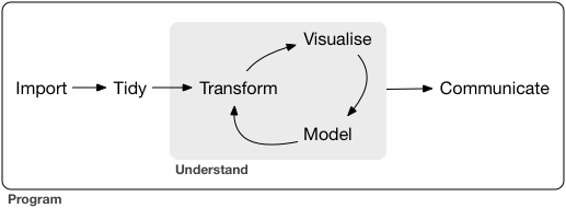
First you must import your data into Python. This typically means that you take data stored in a file, database, or web API, and load it into a data frame in Python. If you can’t get your data into Python, you can’t do data science on it!

Once you’ve imported your data, it is a good idea to tidy it. Tidying your data means storing it in a consistent form that matches the semantics of the dataset with the way it is stored. In brief, when your data is tidy, each column is a variable, and each row is an observation. Tidy data is important because the consistent structure lets you focus your struggle on questions about the data, not fighting to get the data into the right form for different functions.

Once you have tidy data, a common first step is to transform it. Transformation includes narrowing in on observations of interest (like all people in one city, or all data from the last year), creating new variables that are functions of existing variables (like computing speed from distance and time), and calculating a set of summary statistics (like counts or means). Together, tidying and transforming are called wrangling, because getting your data in a form that’s natural to work with often feels like a fight!

Once you have tidy data with the variables you need, there are two main engines of knowledge generation: visualisation and modelling. These have complementary strengths and weaknesses so any real analysis will iterate between them many times.

Visualisation is a fundamentally human activity. A good visualisation will show you things that you did not expect, or raise new questions about the data. A good visualisation might also hint that you’re asking the wrong question, or you need to collect different data. Visualisations can surprise you, but don’t scale particularly well because they require a human to interpret them.

Models are complementary tools to visualisation. Once you have made your questions sufficiently precise, you can use a model to answer them. Models are a fundamentally mathematical or computational tool, so they generally scale well. Even when they don’t, it’s usually cheaper to buy more computers than it is to buy more brains! But every model makes assumptions, and by its very nature a model cannot question its own assumptions. That means a model cannot fundamentally surprise you.

The last step of data science is communication, an absolutely critical part of any data analysis project. It doesn’t matter how well your models and visualisation have led you to understand the data unless you can also communicate your results to others.

Surrounding all these tools is programming. Programming is a cross-cutting tool that you use in every part of the project. You don’t need to be an expert programmer to be a data scientist, but learning more about programming pays off because becoming a better programmer allows you to automate common tasks, and solve new problems with greater ease.

You’ll use these tools in every data science project, but for most projects they’re not enough. There’s a rough 80-20 rule at play; you can tackle about 80% of every project using the tools that you’ll learn in this book, but you’ll need other tools to tackle the remaining 20%. Throughout this book we’ll point you to resources where you can learn more.

1.2 How this book is organised

The previous description of the tools of data science is organised roughly according to the order in which you use them in an analysis (although of course you’ll iterate through them multiple times). In our experience, however, this is not the best way to learn them:

Starting with data ingest and tidying is sub-optimal because 80% of the time it’s routine and boring, and the other 20% of the time it’s weird and frustrating. That’s a bad place to start learning a new subject! Instead, we’ll start with visualisation and transformation of data that’s already been imported and tidied. That way, when you ingest and tidy your own data, your motivation will stay high because you know the pain is worth it.
Some topics are best explained with other tools. For example, we believe that it’s easier to understand how models work if you already know about visualisation, tidy data, and programming.
Programming tools are not necessarily interesting in their own right, but do allow you to tackle considerably more challenging problems. We’ll give you a selection of programming tools in the middle of the book, and then you’ll see how they can combine with the data science tools to tackle interesting modelling problems.

Within each chapter, we try and stick to a similar pattern: start with some motivating examples so you can see the bigger picture, and then dive into the details. Each section of the book is paired with exercises to help you practice what you’ve learned. While it’s tempting to skip the exercises, there’s no better way to learn than practicing on real problems.

1.3 What you won’t learn

There are some important topics that this book doesn’t cover. We believe it’s important to stay ruthlessly focused on the essentials so you can get up and running as quickly as possible. That means this book can’t cover every important topic.

1.3.1 Big data

This book proudly focuses on small, in-memory datasets. This is the right place to start because you can’t tackle big data unless you have experience with small data. The tools you learn in this book will easily handle hundreds of megabytes of data, and with a little care you can typically use them to work with 1-2 Gb of data. If you’re routinely working with larger data (10-100 Gb, say), you should learn more about dask. This book doesn’t teach dask but it is very similar to the pandas workflow. But if you’re working with large data, the performance payoff is worth the extra effort required to learn it.

If your data is bigger than this, carefully consider if your big data problem might actually be a small data problem in disguise. While the complete data might be big, often the data needed to answer a specific question is small. You might be able to find a subset, subsample, or summary that fits in memory and still allows you to answer the question that you’re interested in. The challenge here is finding the right small data, which often requires a lot of iteration.

Another possibility is that your big data problem is actually a large number of small data problems. Each individual problem might fit in memory, but you have millions of them. For example, you might want to fit a model to each person in your dataset. That would be trivial if you had just 10 or 100 people, but instead you have a million. Fortunately each problem is independent of the others (a setup that is sometimes called embarrassingly parallel), so you just need a system (like Hadoop or Spark) that allows you to send different datasets to different computers for processing. Once you’ve figured out how to answer the question for a single subset using the tools described in this book, you learn new tools like sparklyr, rhipe, and ddr to solve it for the full dataset.

1.3.2 R, Julia, and friends

In this book, you won’t learn anything about R, Julia, or any other programming language useful for data science. This isn’t because we think these tools are bad. They’re not! And in practice, most data science teams use a mix of languages, often at least R and Python.

However, we strongly believe that it’s best to master one tool at a time. You will get better faster if you dive deep, rather than spreading yourself thinly over many topics. This doesn’t mean you should only know one thing, just that you’ll generally learn faster if you stick to one thing at a time. You should strive to learn new things throughout your career, but make sure your understanding is solid before you move on to the next interesting thing.

We think Python is a great place to start your data science journey because it is an environment designed from the ground up to support data science. Python is not just a programming language, but it is also an interactive environment for doing data science. To support interaction, Python is a much more flexible language than many of its peers.

1.3.3 Non-rectangular data

This book focuses exclusively on rectangular data: collections of values that are each associated with a variable and an observation. There are lots of datasets that do not naturally fit in this paradigm: including images, sounds, trees, and text. But rectangular data frames are extremely common in science and industry, and we believe that they are a great place to start your data science journey.

1.3.4 Hypothesis confirmation

It’s possible to divide data analysis into two camps: hypothesis generation and hypothesis confirmation (sometimes called confirmatory analysis). The focus of this book is unabashedly on hypothesis generation, or data exploration. Here you’ll look deeply at the data and, in combination with your subject knowledge, generate many interesting hypotheses to help explain why the data behaves the way it does. You evaluate the hypotheses informally, using your scepticism to challenge the data in multiple ways.

The complement of hypothesis generation is hypothesis confirmation. Hypothesis confirmation is hard for two reasons:

You need a precise mathematical model in order to generate falsifiable predictions. This often requires considerable statistical sophistication.
You can only use an observation once to confirm a hypothesis. As soon as you use it more than once you’re back to doing exploratory analysis. This means to do hypothesis confirmation you need to “preregister” (write out in advance) your analysis plan, and not deviate from it even when you have seen the data. We’ll talk a little about some strategies you can use to make this easier in modelling.

It’s common to think about modelling as a tool for hypothesis confirmation, and visualisation as a tool for hypothesis generation. But that’s a false dichotomy: models are often used for exploration, and with a little care you can use visualisation for confirmation. The key difference is how often do you look at each observation: if you look only once, it’s confirmation; if you look more than once, it’s exploration.

1.4 Prerequisites

We’ve made a few assumptions about what you already know in order to get the most out of this book. You should be generally numerically literate, and it’s helpful if you have some programming experience already.

There are four things you need to run the code in this book: Python, VS Code, a package managment system, and a handful of other packages. Packages are the fundamental units of reproducible Python code. They include reusable functions, the documentation that describes how to use them, and sample data.

1.4.1 Python

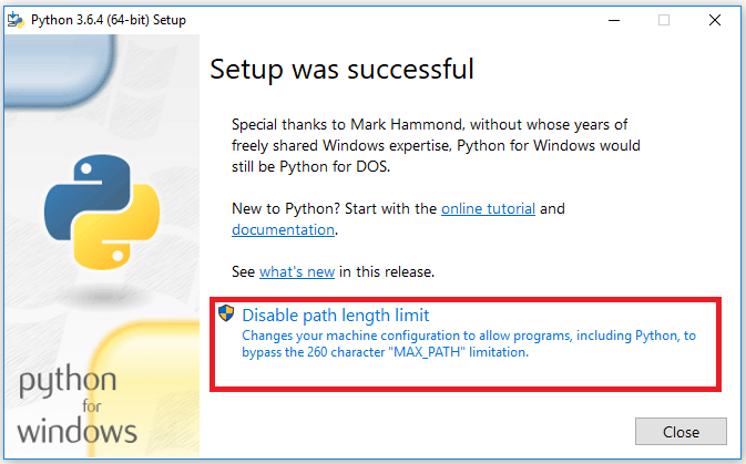
To download Python, go to python.org and download the 64 bit version Python for your OS. A new major version of Python is released every few years, and there are 5-12 minor releases each year.

1.4.1.1 Windows

Make sure to check the box that says, “Add Python ## to PATH”

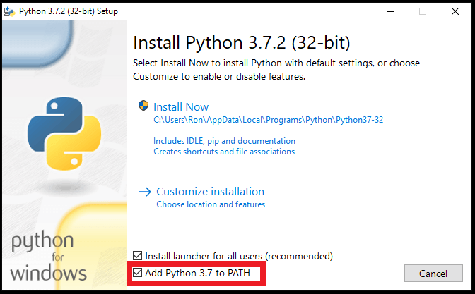
Make sure to click on the “Disable path length limit”

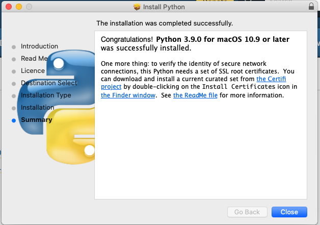
1.4.1.2 Mac

Make sure to Install Certificates so that we can read files from the web. You will see the below window at the last step of installation.

1.4.2 Visual Studio Code (VS Code)

Visual Studio Code is a lightweight but powerful source code editor which runs on your desktop and is available for Windows, macOS and Linux. It comes with built-in support for JavaScript, TypeScript and Node.js and has a rich ecosystem of extensions for other languages (such as C++, C#, Java, Python, PHP, Go) and runtimes (such as .NET and Unity). Begin your journey with VS Code with these introductory videos. Microsoft provides a great overview of VS Code in their docs.

When you use VS code, you’ll have four key regions in the interface:

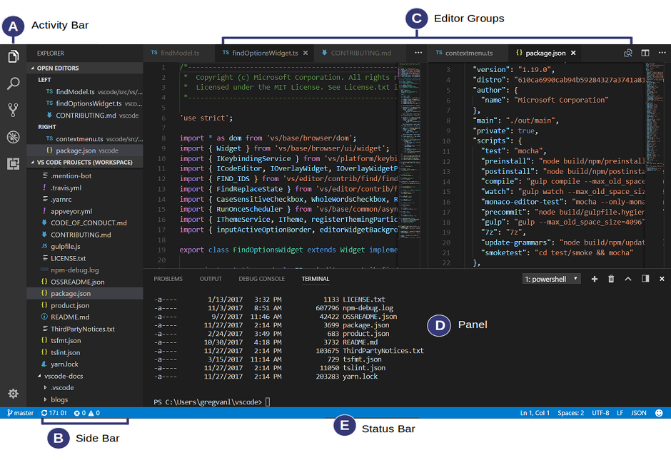
VS Code comes with a simple and intuitive layout that maximizes the space provided for the editor while leaving ample room to browse and access the full context of your folder or project. The UI is divided into five areas:

Editor - The main area to edit your files. You can open as many editors as you like side by side vertically and horizontally.
Side Bar - Contains different views like the Explorer to assist you while working on your project.
Status Bar - Information about the opened project and the files you edit.
Activity Bar - Located on the far left-hand side, this lets you switch between views and gives you additional context-specific indicators, like the number of outgoing changes when Git is enabled.
Panels - You can display different panels below the editor region for output or debug information, errors and warnings, or an integrated terminal. Panel can also be moved to the right for more vertical space. Each time you start VS Code, it opens up in the same state it was in when you last closed it. The folder, layout, and opened files are preserved.

Microsoft provides a great python tutorial and python data science to get you through the following sections if you would like to follow their guides.

1.4.2.1 VS Code Python Extension

Install the Python extension for VS Code from the Visual Studio Marketplace. For additional details on installing extensions, see Extension Marketplace. The Python extension is named Python and it’s published by Microsoft. You can follow more of their tutorial at code.visualstudio.com.

The third video and fourth video in this Python for Beginners set of videos done by Microsoft can also guide you through the Python Extension.

1.4.2.2 VS Code Interactive Python Window

An open-source project called Jupyter is the standard method for interactive Python use for data science or scientific computing. However, there are some issues with its use in a development environment. VS Code has provided a way for us to have the best of Python and Jupyter Notebooks with their Python Interactive Window.

You will need to install the jupyter python package using pip or pip3 for the interactive Python window to work. See the following section for guidance on using pip.

Using the VS Code functionality, you will work with a standard .py file instead of the .ipynb extension typically used with jupyter notebooks. The Python extension in VS Code will recognize # %% as a cell or chunk of python code and add notebook options to ‘Run Cell’ as well as other actions. You can see the code example bellow with the image of the view in VS Code as an example. Microsoft’s documentation goes into more detail (https://code.visualstudio.com/docs/python/jupyter-support-py).

To make the interactive window use more functional you can ctrl + , or cmd + , on a mac to open the settings. From there you can search ‘Send Selection to Interactive Window’ and make sure the box is checked. Now you will be able to use shift + return to send a selected chunk of code or an entire cell.

# %%
msg = "Hello World"
print(msg)

# %%
msg = "Hello again"
print(msg)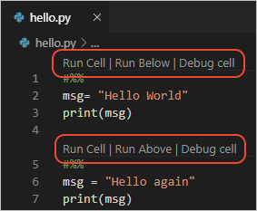

1.4.3 Package Management (pip)

You can install a standard set of data science python packages using pip with your OS command line tools (Mac Terminal, Windos - Command Prompt NOT IN A PYTHON INTERACTIVE ENVIRONMENT). However, there are some complications using pip on computers with multiple versions of Python.

pip: If your path environment is correct, then a standard pip install [package] will work. This is how most packages direct users to install Python packages.
pip3: If your OS has Python 2 and Python 3 installed, you may need to use pip3 install [package].
Force Python version: You can run the pip related to a specific Python installation by using python -m pip install [package]. Some may need to provide the path to their Python installation if your Python path environment is not understood.

A few cautions about package management with pip.

Never run sudo pip install.
If you don’t have root permissions or the OS package manager doesn’t have the package you need, use pip install --user.
If you want multiple versions of the same library to coexist, to do Python development, or to isolate dependencies for any other reason, use virtual environments.
Generally, you will want to update pip before installing packages - python -m pip install --user --upgrade pip setuptools wheel

Conda, poetry, and pipenv are three other options for package management. However, we will focus on using pip.

1.4.3.1 pip package installation examples

If we wanted to install the numpy, pandas, xlrd, matplolib, and seaborn packages, we would use pip. Depending on your OS configuration, one of the following should work.

Everything in your path is clean and you are an admin on your computer

pip install numpy pandas xlrd matplotlib seaborn

Everything in your path is clean and you want to install package for the user

pip install --user numpy pandas xlrd matplotlib seaborn

You have multiple Python versions installed you want to install package for the user without a need to understand which pip maps to which Python

python -m pip install --user numpy pandas xlrd matplotlib seaborn

1.4.4 The Data Science Packages

You’ll also need to install some Python packages. A Python package is a collection of functions, data, and documentation that extends the capabilities of base Python. Using packages is key to the successful use of Python for data science. Note that a Python package can be referred as a Python library as well. The majority of the packages that you will learn in this book are related to the so-called tidyverse packages in R. There are attempts to port they tidyverse package process into Python. We are not showing the tools that recreate the tidyverse in Python but those that current Data Scientists use to do equivelent work in Python. You will notice that pandas is the primary tool with a few packages that come with base Python. Pandas user guide will be referenced heavily as we progress.

R Tidyverse Package	Python Package
dplyr	pandas
tidyr	pandas
tibble	pandas
stringr	string and re
forcats	pandas categorical data
readr	pandas io tools
readxl	xlrd and openpyxl
ggplot2	seaborn, altair, plotnine
purrr	built in map function
base R stats package	statsmodels
tidymodels	scikit-learn
R tensorflow	tensorflow
R keras	keras
rmarkdown	jupyter

Notice that the visualization space in Python does not have a force like ggplot2. Chris Moffitt provided an efficient visualization tools diagram to help Python users with this decision.

The following packages will give us a broad data science toolset in Python.

pip install numpy pandas xlrd matplotlib
pip install seaborn plotnine altair vega_datasets altair_saver
pip install statsmodels scikit-learn
pip install jupyter

On your computer, type that above of code in the command line. The Python package manager pip will download the packages from PyPi and install them on to your computer. If you have problems installing, make sure that you are connected to the internet.

You will not be able to use the functions and objects in a package until you load it with import. It is common in Python for each package to have a standard abbreviated name. For example, numpy is imported as ‘np’, and pandas is imported as ‘pd’ in the code chunk below.

import pandas as pd
import altair as alt
import numpy as np

There are many other excellent packages that are not included here.

1.5 Running Python code

The previous section showed you a couple of examples of running Python code. Code in the book looks like this:

1 + 2
#> 3
#> 3

If you run the same code in interactive python with VS Code, it will look like this:

[1] 1 + 2
3

The Python Interactive window can be used as a standalone console with arbitrary code (with or without code cells). To use the window as a console, open it with the Python: Show Python Interactive window command from the Command Palette. You can then type in code, using Enter to go to a new line and Shift+Enter to run the code.

There are two main differences. In your interactive window, you type after the [#]; we don’t show the line number in the book. In the book, output is commented out with #>; in your console it appears directly after your code. These two differences mean that if you’re working with an electronic version of the book, you can easily copy code out of the book and into the interactive window.

Throughout the book we use a consistent set of conventions to refer to code:

Functions are in a code font and followed by parentheses, like sum(), or mean().
Other Python objects (like data or function arguments) are in a code font, without parentheses, like flights or x.

1.6 Getting help and learning more

This book is not an island; there is no single resource that will allow you to master Python for data science. As you start to apply the techniques described in this book to your own data you will soon find questions that we do not answer. This section describes a few tips on how to get help, and to help you keep learning.

If you get stuck, start with Google. Typically adding “python” to a query is enough to restrict it to relevant results: if the search isn’t useful, it often means that there aren’t any Python-specific results available. Google is particularly useful for error messages. If you get an error message and you have no idea what it means, try googling it! Chances are that someone else has been confused by it in the past, and there will be help somewhere on the web. (If the error message isn’t in English, run Sys.setenv(LANGUAGE = "en") and re-run the code; you’re more likely to find help for English error messages.)

If Google doesn’t help, try stackoverflow. Start by spending a little time searching for an existing answer, including [python] to restrict your search to questions and answers that use Python. If you don’t find anything useful, prepare a minimal reproducible example or reprex. A good reprex makes it easier for other people to help you, and often you’ll figure out the problem yourself in the course of making it.

There are three things you need to include to make your example reproducible: required packages, data, and code.

Packages should be imported at the top of the script, so it’s easy to see which ones the example needs. This is a good time to check that you’re using the latest version of each package; it’s possible you’ve discovered a bug that’s been fixed since you installed the package.
The easiest way to include data in a question is to create a minimal example to that recreates it. Try and find the smallest subset of your data that still reveals the problem.
Spend a little bit of time ensuring that your code is easy for others to read:
- Make sure you’ve used spaces and your variable names are concise, yet informative.
- Use comments to indicate where your problem lies.
- Do your best to remove everything that is not related to the problem. The shorter your code is, the easier it is to understand, and the easier it is to fix.

Finish by checking that you have actually made a reproducible example by starting a fresh Python session to run your script in.

You should also spend some time preparing yourself to solve problems before they occur. Investing a little time in learning Python each day will pay off handsomely in the long run. One way is to follow what Wes McKinney, Garrett, and everyone else at RStudio are doing on the Pandas blog or the ossdata blog. This is where they post announcements about new packages and new IDE features. You might also want to follow Wes McKinney (@wesmckinn) on Twitter, or follow @code to keep up with new features in VS Code.

To keep up with the data science community more broadly, we recommend reading https://planet.scipy.org/#. If you’re an active Twitter user, follow the #datascience hashtag.

1.7 Datasets access

The data used in R for Data Science is generally within the R packages themselves. Many of the Python data science packages also come with datasets upon import. However, we will use the original datasets presented in R for Data Science. We have a data4python4ds GitHub data repository that contains all the datasets in varied file formats and all examples will use Pandas to read the data from GitHub.

1.8 Acknowledgements

The text of this book is largely the product of Hadley and Garrett. J. Hathaway has ported the code and descriptions for using VS Code with help from Katie Larson. You can see the original acknowledgements here.

1.9 Colophon

An online version of this book is available at https://byuidatascience.github.io/python4ds/. It will continue to evolve. The source of the book is available at https://github.com/byuidatascience/python4ds. The book is powered by https://bookdown.org which makes it easy to turn R markdown files into HTML, PDF, and EPUB.

This book was built with:

sessioninfo::session_info()
#> ─ Session info ───────────────────────────────────────────────────────────────
#>  setting  value                       
#>  version  R version 4.0.4 (2021-02-15)
#>  os       macOS Big Sur 10.16         
#>  system   x86_64, darwin17.0          
#>  ui       X11                         
#>  language (EN)                        
#>  collate  en_US.UTF-8                 
#>  ctype    en_US.UTF-8                 
#>  tz       America/Boise               
#>  date     2021-04-21                  
#> 
#> ─ Packages ───────────────────────────────────────────────────────────────────
#>  package     * version   date       lib source                             
#>  bookdown      0.21.7    2021-03-30 [1] Github (rstudio/bookdown@f7d0622)  
#>  cli           2.4.0     2021-04-05 [1] CRAN (R 4.0.2)                     
#>  colorspace    2.0-0     2020-11-11 [1] CRAN (R 4.0.2)                     
#>  crayon        1.4.1     2021-02-08 [1] CRAN (R 4.0.2)                     
#>  digest        0.6.27    2020-10-24 [1] CRAN (R 4.0.2)                     
#>  dplyr         1.0.2     2020-08-18 [1] CRAN (R 4.0.2)                     
#>  ellipsis      0.3.1     2020-05-15 [1] CRAN (R 4.0.2)                     
#>  evaluate      0.14      2019-05-28 [1] CRAN (R 4.0.1)                     
#>  fansi         0.4.2     2021-01-15 [1] CRAN (R 4.0.2)                     
#>  generics      0.1.0     2020-10-31 [1] CRAN (R 4.0.2)                     
#>  ggplot2     * 3.3.3     2020-12-30 [1] CRAN (R 4.0.2)                     
#>  glue          1.4.2     2020-08-27 [1] CRAN (R 4.0.2)                     
#>  gtable        0.3.0     2019-03-25 [1] CRAN (R 4.0.2)                     
#>  highr         0.8       2019-03-20 [1] CRAN (R 4.0.2)                     
#>  htmltools     0.5.1.1   2021-01-22 [1] CRAN (R 4.0.2)                     
#>  jsonlite      1.7.2     2020-12-09 [1] CRAN (R 4.0.2)                     
#>  knitr         1.31      2021-01-27 [1] CRAN (R 4.0.2)                     
#>  lattice       0.20-41   2020-04-02 [1] CRAN (R 4.0.4)                     
#>  lifecycle     1.0.0     2021-02-15 [1] CRAN (R 4.0.2)                     
#>  magrittr      2.0.1     2020-11-17 [1] CRAN (R 4.0.2)                     
#>  Matrix        1.3-2     2021-01-06 [1] CRAN (R 4.0.4)                     
#>  munsell       0.5.0     2018-06-12 [1] CRAN (R 4.0.2)                     
#>  pillar        1.5.1     2021-03-05 [1] CRAN (R 4.0.2)                     
#>  pkgconfig     2.0.3     2019-09-22 [1] CRAN (R 4.0.2)                     
#>  purrr         0.3.4     2020-04-17 [1] CRAN (R 4.0.2)                     
#>  R6            2.5.0     2020-10-28 [1] CRAN (R 4.0.2)                     
#>  Rcpp          1.0.6     2021-01-15 [1] CRAN (R 4.0.2)                     
#>  reticulate  * 1.18-9008 2021-04-05 [1] Github (rstudio/reticulate@1aff9d8)
#>  rlang         0.4.10    2020-12-30 [1] CRAN (R 4.0.2)                     
#>  rmarkdown     2.7.4     2021-03-30 [1] Github (rstudio/rmarkdown@a11240d) 
#>  scales        1.1.1     2020-05-11 [1] CRAN (R 4.0.2)                     
#>  sessioninfo   1.1.1     2018-11-05 [1] CRAN (R 4.0.2)                     
#>  stringi       1.5.3     2020-09-09 [1] CRAN (R 4.0.2)                     
#>  stringr       1.4.0     2019-02-10 [1] CRAN (R 4.0.2)                     
#>  tibble        3.1.0     2021-02-25 [1] CRAN (R 4.0.2)                     
#>  tidyselect    1.1.0     2020-05-11 [1] CRAN (R 4.0.2)                     
#>  utf8          1.2.1     2021-03-12 [1] CRAN (R 4.0.2)                     
#>  vctrs         0.3.7     2021-03-29 [1] CRAN (R 4.0.2)                     
#>  withr         2.4.1     2021-01-26 [1] CRAN (R 4.0.2)                     
#>  xfun          0.22      2021-03-11 [1] CRAN (R 4.0.2)                     
#>  yaml          2.2.1     2020-02-01 [1] CRAN (R 4.0.2)                     
#> 
#> [1] /Library/Frameworks/R.framework/Versions/4.0/Resources/library