12 Tidy data

12.1 Introduction

“Happy families are all alike; every unhappy family is unhappy in its own way.” –– Leo Tolstoy

“Tidy datasets are all alike, but every messy dataset is messy in its own way.” –– Hadley Wickham

In this chapter, you will learn a consistent way to organise your data in Python, an organisation called tidy data. Getting your data into this format requires some upfront work, but that work pays off in the long term. Once you have tidy data and pandas data frames, you will spend much less time munging data from one representation to another, allowing you to spend more time on the analytic questions at hand.

This chapter will give you a practical introduction to tidy data and the accompanying tools in the pandas package. If you’d like to learn more about the underlying theory, you might enjoy the Tidy Data article published in the Journal of Statistical Software.

12.1.1 Prerequisites

In this chapter we’ll focus on pandas, a package that provides a bunch of tools to help tidy up your messy datasets.

import pandas as pd
import altair as alt
import numpy as np

12.2 Tidy data

You can represent the same underlying data in multiple ways. The example below shows the same data organised in four different ways. Each dataset shows the same values of four variables country, year, population, and cases, but each dataset organises the values in a different way.

base_url = "https://github.com/byuidatascience/data4python4ds/raw/master/data-raw/"
table1 = pd.read_csv("{}table1/table1.csv".format(base_url))
table2 = pd.read_csv("{}table2/table2.csv".format(base_url))
table3 = pd.read_csv("{}table3/table3.csv".format(base_url))
table4a = pd.read_csv("{}table4a/table4a.csv".format(base_url))
table4b = pd.read_csv("{}table4b/table4b.csv".format(base_url))
table5 = pd.read_csv("{}table5/table5.csv".format(base_url), dtype = 'object')

table1
#>        country  year   cases  population
#> 0  Afghanistan  1999     745    19987071
#> 1  Afghanistan  2000    2666    20595360
#> 2       Brazil  1999   37737   172006362
#> 3       Brazil  2000   80488   174504898
#> 4        China  1999  212258  1272915272
#> 5        China  2000  213766  1280428583
table2
#>         country  year        type       count
#> 0   Afghanistan  1999       cases         745
#> 1   Afghanistan  1999  population    19987071
#> 2   Afghanistan  2000       cases        2666
#> 3   Afghanistan  2000  population    20595360
#> 4        Brazil  1999       cases       37737
#> 5        Brazil  1999  population   172006362
#> 6        Brazil  2000       cases       80488
#> 7        Brazil  2000  population   174504898
#> 8         China  1999       cases      212258
#> 9         China  1999  population  1272915272
#> 10        China  2000       cases      213766
#> 11        China  2000  population  1280428583
table3

# Spread across two tibbles
#>        country  year               rate
#> 0  Afghanistan  1999       745/19987071
#> 1  Afghanistan  2000      2666/20595360
#> 2       Brazil  1999    37737/172006362
#> 3       Brazil  2000    80488/174504898
#> 4        China  1999  212258/1272915272
#> 5        China  2000  213766/1280428583
table4a  # cases
#>        country    1999    2000
#> 0  Afghanistan     745    2666
#> 1       Brazil   37737   80488
#> 2        China  212258  213766
table4b  # population
#>        country        1999        2000
#> 0  Afghanistan    19987071    20595360
#> 1       Brazil   172006362   174504898
#> 2        China  1272915272  1280428583

These are all representations of the same underlying data, but they are not equally easy to use. One dataset, the tidy dataset, will be much easier to work with inside the tidyverse.

There are three interrelated rules which make a dataset tidy:

Each variable must have its own column.
Each observation must have its own row.
Each value must have its own cell.

Figure 12.1 shows the rules visually.

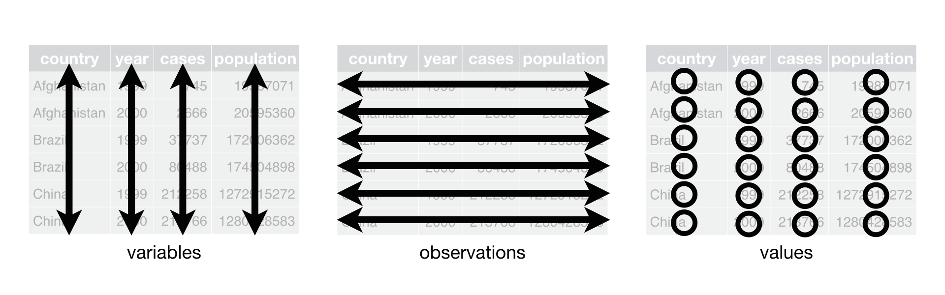
Figure 12.1: Following three rules makes a dataset tidy: variables are in columns, observations are in rows, and values are in cells.

These three rules are interrelated because it’s impossible to only satisfy two of the three. That interrelationship leads to an even simpler set of practical instructions:

Put each dataset in a tibble.
Put each variable in a column.

In this example, only table1 is tidy. It’s the only representation where each column is a variable.

Why ensure that your data is tidy? There are two main advantages:

There’s a general advantage to picking one consistent way of storing data. If you have a consistent data structure, it’s easier to learn the tools that work with it because they have an underlying uniformity.
There’s a specific advantage to placing variables in columns because it allows pandas’ and NumPy’s vectorised nature to shine. As you learned in assign and aggregate functions, most built-in R functions work with vectors of values. That makes transforming tidy data feel particularly natural.

Altair and pandas work well with tidy data. Here are a couple of small examples showing how you might work with table1.

# Compute rate per 10,000
table1.assign(
    rate = lambda x: x.cases / x.population * 1000
)
# Compute cases per year
#>        country  year   cases  population      rate
#> 0  Afghanistan  1999     745    19987071  0.037274
#> 1  Afghanistan  2000    2666    20595360  0.129447
#> 2       Brazil  1999   37737   172006362  0.219393
#> 3       Brazil  2000   80488   174504898  0.461236
#> 4        China  1999  212258  1272915272  0.166750
#> 5        China  2000  213766  1280428583  0.166949
(table1.
  groupby('year').
  agg(n = ('cases', 'sum')).
  reset_index())

# Visualise changes over time
# import altair as alt
#>    year       n
#> 0  1999  250740
#> 1  2000  296920
base_chart = (alt.Chart(table1).
  encode(alt.X('year'), alt.Y('cases'), detail = 'country'))

chart = base_chart.mark_line() + base_chart.encode(color = 'country').mark_circle()

chart.save("screenshots/altair_table1.png")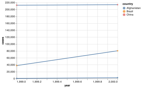

12.2.1 Exercises

Using prose, describe how the variables and observations are organised in each of the sample tables.
Compute the rate for table2, and table4a + table4b. You will need to perform four operations:
1. Extract the number of TB cases per country per year.
2. Extract the matching population per country per year.
3. Divide cases by population, and multiply by 10000.
4. Store back in the appropriate place.
Which representation is easiest to work with? Which is hardest? Why?
Recreate the plot showing change in cases over time using table2 instead of table1. What do you need to do first?

12.3 Pivoting

The principles of tidy data seem so obvious that you might wonder if you’ll ever encounter a dataset that isn’t tidy. Unfortunately, however, most data that you will encounter will be untidy. There are two main reasons:

Most people aren’t familiar with the principles of tidy data, and it’s hard to derive them yourself unless you spend a lot of time working with data.
Data is often organised to facilitate some use other than analysis. For example, data is often organised to make entry as easy as possible.

This means for most real analyses, you’ll need to do some tidying. The first step is always to figure out what the variables and observations are. Sometimes this is easy; other times you’ll need to consult with the people who originally generated the data.

The second step is to resolve one of two common problems:

One variable might be spread across multiple columns.
One observation might be scattered across multiple rows.

Typically a dataset will only suffer from one of these problems; it’ll only suffer from both if you’re really unlucky! To fix these problems, you’ll need two functions in pandas: melt(), pivot(), and pivot_table(). There are two additional functions called stack() and unstack() that use multi-index columns and rows. Pandas provides a guide to reshaping and pivot tables in their user guide.

12.3.1 Longer (`melt()`)

A common problem is a dataset where some of the column names are not names of variables, but values of a variable. Take table4a: the column names 1999 and 2000 represent values of the year variable, the values in the 1999 and 2000 columns represent values of the cases variable, and each row represents two observations, not one.

table4a
#>        country    1999    2000
#> 0  Afghanistan     745    2666
#> 1       Brazil   37737   80488
#> 2        China  212258  213766

To tidy a dataset like this, we need to stack the offending columns into a new pair of variables. To describe that operation we need three parameters:

The set of columns whose names are identifier variables, not values. In this example, country is the identifier column and the value columns are 1999 and 2000.
The name of the variable to move the column names to. Here it is year.
The name of the variable to move the column values to. Here it’s cases.

Together those parameters generate the call to melt():

table4a.melt(['country'], var_name = "year", value_name = "cases")
#>        country  year   cases
#> 0  Afghanistan  1999     745
#> 1       Brazil  1999   37737
#> 2        China  1999  212258
#> 3  Afghanistan  2000    2666
#> 4       Brazil  2000   80488
#> 5        China  2000  213766

year and cases do not exist in table4a so we put their names in quotes.

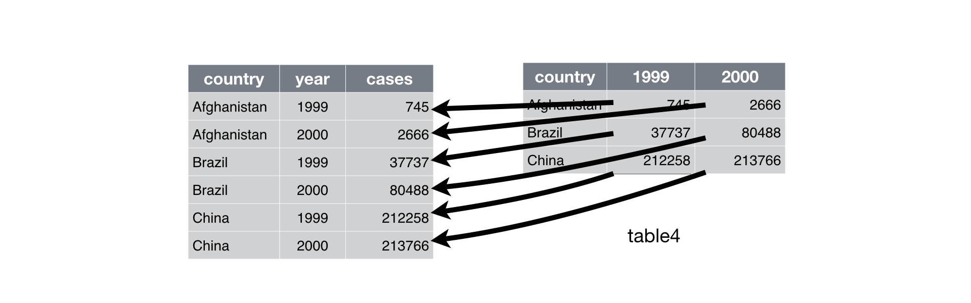
Figure 12.2: Pivoting table4 into a longer, tidy form.

In the final result, the pivoted columns are dropped, and we get new year and cases columns. Otherwise, the relationships between the original variables are preserved. Visually, this is shown in Figure 12.2.

melt() makes datasets longer (imagine melting icecream down the cone) by increasing the number of rows and decreasing the number of columns. I don’t believe it makes sense to describe a dataset as being in “long form”. Length is a relative term, and you can only say that dataset A is longer than dataset B.

We can use melt() to tidy table4b in a similar fashion. The only difference is the variable stored in the cell values:

table4b.melt(['country'], var_name = 'year', value_name = 'population')
#>        country  year  population
#> 0  Afghanistan  1999    19987071
#> 1       Brazil  1999   172006362
#> 2        China  1999  1272915272
#> 3  Afghanistan  2000    20595360
#> 4       Brazil  2000   174504898
#> 5        China  2000  1280428583

To combine the tidied versions of table4a and table4b into a single tibble, we need to use merge(), which you’ll learn about in relational data.

tidy4a = table4a.melt(['country'], var_name = "year", value_name = "cases")
tidy4b = table4b.melt(['country'], var_name = 'year', value_name = 'population')
pd.merge(tidy4a, tidy4b, on = ['country', 'year'])
#>        country  year   cases  population
#> 0  Afghanistan  1999     745    19987071
#> 1       Brazil  1999   37737   172006362
#> 2        China  1999  212258  1272915272
#> 3  Afghanistan  2000    2666    20595360
#> 4       Brazil  2000   80488   174504898
#> 5        China  2000  213766  1280428583

12.3.2 Wider (`pivot()`)

pivot() is the opposite of melt(). You use it when an observation is scattered across multiple rows. For example, take table2: an observation is a country in a year, but each observation is spread across two rows.

table2
#>         country  year        type       count
#> 0   Afghanistan  1999       cases         745
#> 1   Afghanistan  1999  population    19987071
#> 2   Afghanistan  2000       cases        2666
#> 3   Afghanistan  2000  population    20595360
#> 4        Brazil  1999       cases       37737
#> 5        Brazil  1999  population   172006362
#> 6        Brazil  2000       cases       80488
#> 7        Brazil  2000  population   174504898
#> 8         China  1999       cases      212258
#> 9         China  1999  population  1272915272
#> 10        China  2000       cases      213766
#> 11        China  2000  population  1280428583

To tidy this up, we first analyse the representation in similar way to melt(). This time, however, we only need two parameters:

The column to take variable names from. Here, it’s type.
The column to take values from. Here it’s count.

Once we’ve figured that out, we can use pivot(), as shown programmatically below, and visually in Figure 12.3.

In this example, we have a multi-column index argument and will need to use pivot_table(). With a single column index pivot() can be used.

table2.pivot_table(
    index = ['country', 'year'], 
    columns = 'type', 
    values = 'count').reset_index()
#> type      country  year   cases  population
#> 0     Afghanistan  1999     745    19987071
#> 1     Afghanistan  2000    2666    20595360
#> 2          Brazil  1999   37737   172006362
#> 3          Brazil  2000   80488   174504898
#> 4           China  1999  212258  1272915272
#> 5           China  2000  213766  1280428583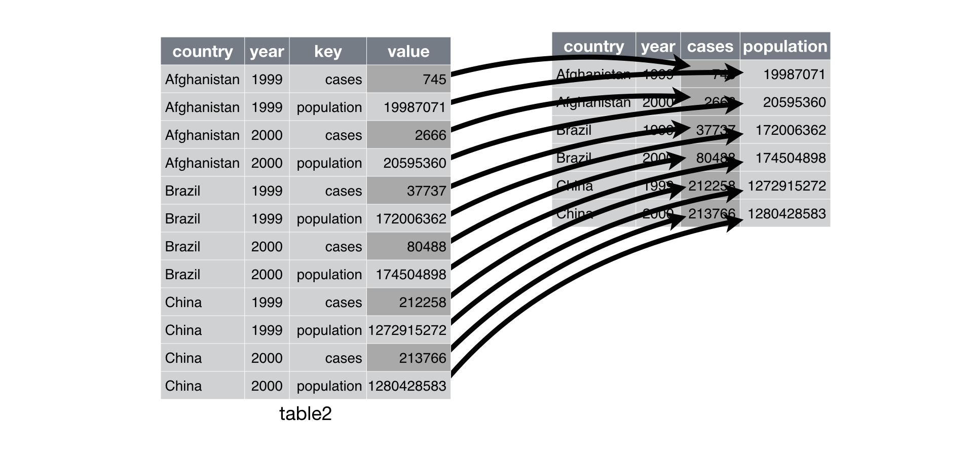

Figure 12.3: Pivoting table2 into a “wider”, tidy form.

As you might have guessed from their names, pivot() and pivot_table() are complements to melt(). melt() makes wide tables narrower and longer; pivot() and pivot_table() makes long tables shorter and wider.

12.3.3 Exercises

Why are melt() and pivot() not perfectly symmetrical? Carefully consider the following example:

stocks = pd.DataFrame({
  'year': [2015, 2015, 2016, 2016],
  'half':  [1,    2,     1,    2],
  'return': [1.88, 0.59, 0.92, 0.17]
})
(stocks.
  pivot(
    index = 'half', 
    columns = 'year', 
    values = 'return').
  melt(
    var_name = 'year', 
    value_name = 'return')
  )

(Hint: look at the variable types and think about column names.)

12.4 Separating and uniting

So far you’ve learned how to tidy table2 and table4, but not table3. table3 has a different problem: we have one column (rate) that contains two variables (cases and population). To fix this problem, we’ll need the pandas str.split() function. You’ll also learn about the complement of str.split(): str.join(), which you use if a single variable is spread across multiple columns.

12.4.1 Split (Separate)

str.split() pulls apart one column into multiple columns, by splitting wherever a separator character appears. Take table3:

table3
#>        country  year               rate
#> 0  Afghanistan  1999       745/19987071
#> 1  Afghanistan  2000      2666/20595360
#> 2       Brazil  1999    37737/172006362
#> 3       Brazil  2000    80488/174504898
#> 4        China  1999  212258/1272915272
#> 5        China  2000  213766/1280428583

The rate column contains both cases and population variables, and we need to split it into two variables. str.split() takes the name of the column to split. The names of the columns to separate into can be names using rename(), as shown in Figure 12.4 and the code below.

By default, str.split() will split values on white spaces. If you wish to use a specific character to separate a column, you can pass the character to the pat or first argument of str.split().

Unlike tidyr::separate() in R, you will need to append the new columns back onto your data set with a pd.concat() with the argument axis = 1

new_columns = (table3.
  rate.str.split("/", expand = True).
  rename(columns = {0: "cases", 1: "population"})
  )
  
pd.concat([table3.drop(columns = 'rate'), new_columns], axis = 1)
#>        country  year   cases  population
#> 0  Afghanistan  1999     745    19987071
#> 1  Afghanistan  2000    2666    20595360
#> 2       Brazil  1999   37737   172006362
#> 3       Brazil  2000   80488   174504898
#> 4        China  1999  212258  1272915272
#> 5        China  2000  213766  1280428583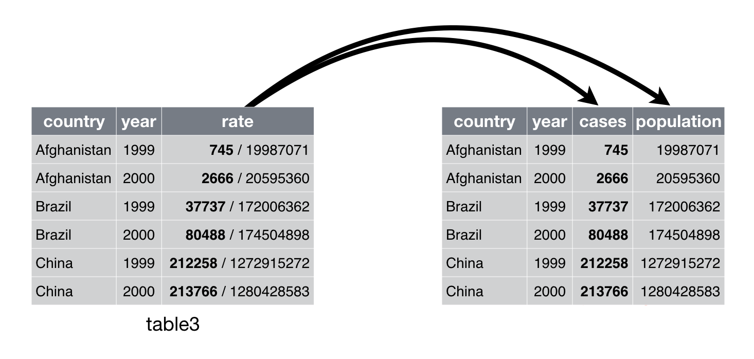

Figure 12.4: Separating table3 makes it tidy

(Formally, pat is a regular expression, which you’ll learn more about in strings.)

Look carefully at the column types: you’ll notice that cases and population are objects or strings. This is the default behaviour in str.split(): it only works on object types and returns objects. Here, however, it’s not very useful as those really are numbers. We can ask use astype() to convert to better types:

pd.concat([
  table3.drop(columns = 'rate'), 
  new_columns.astype('float')],
  axis = 1)
#>        country  year     cases    population
#> 0  Afghanistan  1999     745.0  1.998707e+07
#> 1  Afghanistan  2000    2666.0  2.059536e+07
#> 2       Brazil  1999   37737.0  1.720064e+08
#> 3       Brazil  2000   80488.0  1.745049e+08
#> 4        China  1999  212258.0  1.272915e+09
#> 5        China  2000  213766.0  1.280429e+09

To split on integers you would use str[]. str[] will interpret the integers as positions to split at. Positive values start at 1 on the far-left of the strings and are entered :2; negative value start at -1 on the far-right of the strings are entered -2:.

You can use this arrangement to separate the last two digits of each year. The data will be less tidy, but it is useful in other cases—as you’ll see soon.

cent_year = pd.DataFrame({
    'century': table3.year.astype(str).str[:2],
    'year': table3.year.astype(str).str[-2:]
})

pd.concat([table3.drop(columns = 'year'), cent_year], axis = 1)

#>        country               rate century year
#> 0  Afghanistan       745/19987071      19   99
#> 1  Afghanistan      2666/20595360      20   00
#> 2       Brazil    37737/172006362      19   99
#> 3       Brazil    80488/174504898      20   00
#> 4        China  212258/1272915272      19   99
#> 5        China  213766/1280428583      20   00

12.4.2 Unite

For two string series the inverse of str.split() can be done with +: it combines multiple columns into a single column. You’ll need it much less frequently than str.split(), but it’s still a useful tool to have in your back pocket.

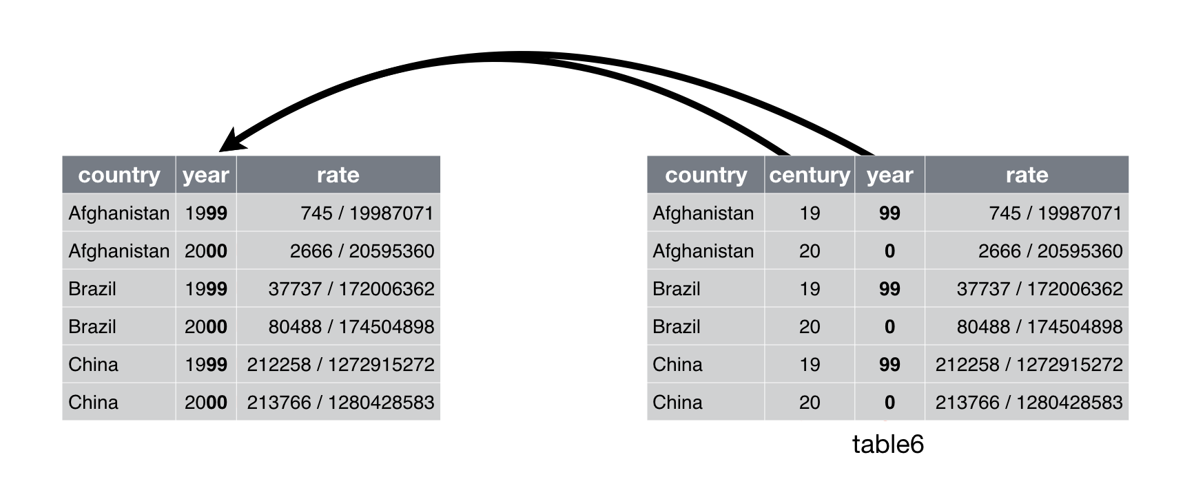
Figure 12.5: Uniting table5 makes it tidy

We can use + to rejoin the century and year string columns that we created in the last example. That data is saved as table5. + takes a two series and can be assigned to the name of the new variable to create:

table5.assign(new = table5['century'] + table5['year'])
#>        country century year               rate   new
#> 0  Afghanistan      19   99       745/19987071  1999
#> 1  Afghanistan      20   00      2666/20595360  2000
#> 2       Brazil      19   99    37737/172006362  1999
#> 3       Brazil      20   00    80488/174504898  2000
#> 4        China      19   99  212258/1272915272  1999
#> 5        China      20   00  213766/1280428583  2000

If you want join the strings with a specified string or more than two columns you can use agg with axis = 1.

table5.assign(new = table5[['century', 'year']].agg("_".join, axis = 1))
#>        country century year               rate    new
#> 0  Afghanistan      19   99       745/19987071  19_99
#> 1  Afghanistan      20   00      2666/20595360  20_00
#> 2       Brazil      19   99    37737/172006362  19_99
#> 3       Brazil      20   00    80488/174504898  20_00
#> 4        China      19   99  212258/1272915272  19_99
#> 5        China      20   00  213766/1280428583  20_00

12.4.3 Exercises

Compare and contrast str.split() and str.extract(). Why are there three variations of separation (by position, by separator, and with groups?

12.5 Missing values

Changing the representation of a dataset brings up an important subtlety of missing values. Surprisingly, a value can be missing in one of two possible ways:

Explicitly, i.e. flagged with nan.
Implicitly, i.e. simply not present in the data.

Let’s illustrate this idea with a very simple data set:

stocks = pd.DataFrame({
    'year': [2015, 2015, 2015, 2015, 2016, 2016, 2016],
    'qtr': [   1,    2,    3,    4,    2,    3,    4],
    'return': [1.88, 0.59, 0.35,   np.nan, 0.92, 0.17, 2.66]
    })

There are two missing values in this dataset:

The return for the fourth quarter of 2015 is explicitly missing, because the cell where its value should be instead contains nan.
The return for the first quarter of 2016 is implicitly missing, because it simply does not appear in the dataset.

One way to think about the difference is with this Zen-like koan: An explicit missing value is the presence of an absence; an implicit missing value is the absence of a presence.

The way that a dataset is represented can make implicit values explicit. For example, we can make the implicit missing value explicit by putting years in the columns:

stocks.pivot(
  index = 'qtr', 
  columns = 'year', 
  values = 'return').reset_index()
#> year  qtr  2015  2016
#> 0       1  1.88   NaN
#> 1       2  0.59  0.92
#> 2       3  0.35  0.17
#> 3       4   NaN  2.66

Because these explicit missing values may not be important in other representations of the data, you turn explicit missing values implicit with .dropna():

stocks.pivot(
  index = 'qtr', 
  columns = 'year', 
  values = 'return').reset_index().melt(id_vars = ['qtr']).dropna()
#>    qtr  year  value
#> 0    1  2015   1.88
#> 1    2  2015   0.59
#> 2    3  2015   0.35
#> 5    2  2016   0.92
#> 6    3  2016   0.17
#> 7    4  2016   2.66

You can use the pandas functions stack() and unstack() with set_index() to take a set of columns and find all unique combinations. This ensures the original dataset contains all values by filling in explicit missingness where necessary. See this stackoverflow for an example. tidyr::complete() in R performs a similar function.

12.6 Case Study

To finish off the chapter, let’s pull together everything you’ve learned to tackle a realistic data tidying problem. The tidyr::who dataset contains tuberculosis (TB) cases broken down by year, country, age, gender, and diagnosis method. The data comes from the 2014 World Health Organization Global Tuberculosis Report.

There’s a wealth of epidemiological information in this dataset, but it’s challenging to work with the data in the form that it’s provided:

who = pd.read_csv("https://github.com/byuidatascience/data4python4ds/raw/master/data-raw/who/who.csv")
# Fix the Namibia NA iso code.
who.loc[who.iso2.isna(),'iso2'] = "NA"

This is a very typical real-life example dataset. It contains redundant columns, odd variable codes, and many missing values. In short, who is messy, and we’ll need multiple steps to tidy it. Pandas is designed so that each function does one thing well. That means in real-life situations you’ll usually need to string together multiple verbs into a pipeline.

The best place to start is almost always to gather together the columns that are not variables. Let’s have a look at what we’ve got:

It looks like country, iso2, and iso3 are three variables that redundantly specify the country.
year is clearly also a variable.
We don’t know what all the other columns are yet, but given the structure in the variable names (e.g. new_sp_m014, new_ep_m014, new_ep_f014) these are likely to be values, not variables.

So we need to gather together all the columns from new_sp_m014 to newrel_f65. We don’t know what those values represent yet, so we’ll give them the generic name "key". We know the cells represent the count of cases, so we’ll use the variable cases. There are a lot of missing values in the current representation, so for now we’ll use na.rm just so we can focus on the values that are present.

who1 = who.melt(
    id_vars = ['country', 'iso2', 'iso3', 'year'], 
    var_name = 'key', 
    value_name = 'cases').dropna()

We can get some hint of the structure of the values in the new key column by counting them:

who1.key.value_counts().head(25)
#> new_sp_m4554    3223
#> new_sp_m3544    3219
#> new_sp_m5564    3218
#> new_sp_m65      3209
#> new_sp_m1524    3209
#> new_sp_m2534    3206
#> new_sp_f4554    3204
#> new_sp_f2534    3200
#> new_sp_f3544    3199
#> new_sp_f65      3197
#> new_sp_f5564    3195
#> new_sp_f1524    3194
#> new_sp_f014     3174
#> new_sp_m014     3173
#> new_sn_m014     1045
#> new_sn_f014     1040
#> new_ep_m014     1038
#> new_ep_f014     1032
#> new_sn_m1524    1030
#> new_sn_m4554    1027
#> new_ep_m1524    1026
#> new_sn_m3544    1025
#> new_ep_m3544    1024
#> new_sn_m2534    1022
#> new_sn_f1524    1022
#> Name: key, dtype: int64

You might be able to parse this out by yourself with a little thought and some experimentation, but luckily we have the data dictionary handy. It tells us:

The first three letters of each column denote whether the column contains new or old cases of TB. In this dataset, each column contains new cases.
The next two letters describe the type of TB:
- rel stands for cases of relapse
- ep stands for cases of extrapulmonary TB
- sn stands for cases of pulmonary TB that could not be diagnosed by a pulmonary smear (smear negative)
- sp stands for cases of pulmonary TB that could be diagnosed be a pulmonary smear (smear positive)
The sixth letter gives the sex of TB patients. The dataset groups cases by males (m) and females (f).
The remaining numbers gives the age group. The dataset groups cases into seven age groups:
- 014 = 0 – 14 years old
- 1524 = 15 – 24 years old
- 2534 = 25 – 34 years old
- 3544 = 35 – 44 years old
- 4554 = 45 – 54 years old
- 5564 = 55 – 64 years old
- 65 = 65 or older

We need to make a minor fix to the format of the column names: unfortunately the names are slightly inconsistent because instead of new_rel we have newrel (it’s hard to spot this here but if you don’t fix it we’ll get errors in subsequent steps). You’ll learn about str.replace() in strings, but the basic idea is pretty simple: replace the characters “newrel” with “new_rel”. This makes all variable names consistent.

who2 = who1.assign(names_from = lambda x: x.key.str.replace('newrel', 'new_rel'))
who2
#>                           country iso2 iso3  ...          key   cases   names_from
#> 17                    Afghanistan   AF  AFG  ...  new_sp_m014     0.0  new_sp_m014
#> 18                    Afghanistan   AF  AFG  ...  new_sp_m014    30.0  new_sp_m014
#> 19                    Afghanistan   AF  AFG  ...  new_sp_m014     8.0  new_sp_m014
#> 20                    Afghanistan   AF  AFG  ...  new_sp_m014    52.0  new_sp_m014
#> 21                    Afghanistan   AF  AFG  ...  new_sp_m014   129.0  new_sp_m014
#> ...                           ...  ...  ...  ...          ...     ...          ...
#> 405269                   Viet Nam   VN  VNM  ...   newrel_f65  3110.0  new_rel_f65
#> 405303  Wallis and Futuna Islands   WF  WLF  ...   newrel_f65     2.0  new_rel_f65
#> 405371                      Yemen   YE  YEM  ...   newrel_f65   360.0  new_rel_f65
#> 405405                     Zambia   ZM  ZMB  ...   newrel_f65   669.0  new_rel_f65
#> 405439                   Zimbabwe   ZW  ZWE  ...   newrel_f65   725.0  new_rel_f65
#> 
#> [76046 rows x 7 columns]

We can separate the values in each code with two passes of str.split(). The first pass will split the codes at each underscore.

new_columns = (who2.names_from.
    str.split("_",expand = True).
    rename(columns = {0: "new", 1: "type", 2: "sexage"}))
new_columns
#>         new type sexage
#> 17      new   sp   m014
#> 18      new   sp   m014
#> 19      new   sp   m014
#> 20      new   sp   m014
#> 21      new   sp   m014
#> ...     ...  ...    ...
#> 405269  new  rel    f65
#> 405303  new  rel    f65
#> 405371  new  rel    f65
#> 405405  new  rel    f65
#> 405439  new  rel    f65
#> 
#> [76046 rows x 3 columns]

Then we might as well drop the new column because it’s constant in this dataset. While we’re dropping columns, let’s also drop iso2 and iso3 since they’re redundant.

# who3 is in R process. They also have an error and they are not using the names_from column.
who4 = pd.concat([
  who2.filter(items = ['country', 'year']),
  new_columns.filter(items = ['type'])], axis = 1)

Next we’ll separate sexage into sex and age by splitting after the first character:

who5 = who4.assign(
  sex = new_columns.sexage.str[:1],
  age = new_columns.sexage.str.slice(1)
)

who5
#>                           country  year type sex  age
#> 17                    Afghanistan  1997   sp   m  014
#> 18                    Afghanistan  1998   sp   m  014
#> 19                    Afghanistan  1999   sp   m  014
#> 20                    Afghanistan  2000   sp   m  014
#> 21                    Afghanistan  2001   sp   m  014
#> ...                           ...   ...  ...  ..  ...
#> 405269                   Viet Nam  2013  rel   f   65
#> 405303  Wallis and Futuna Islands  2013  rel   f   65
#> 405371                      Yemen  2013  rel   f   65
#> 405405                     Zambia  2013  rel   f   65
#> 405439                   Zimbabwe  2013  rel   f   65
#> 
#> [76046 rows x 5 columns]

The who dataset is now ‘kinda’ tidy! We have left the age range as age for simplicity.

I’ve shown you the code a piece at a time, assigning each interim result to a new variable. This typically isn’t how you’d work interactively. Instead, you’d use as little assignment as possible:

# assigned fixed values back into key this time.
who_melt = who.melt(
    id_vars = ['country', 'iso2', 'iso3', 'year'], 
    var_name = 'key', 
    value_name = 'cases').dropna().assign(
        key = lambda x: x.key.str.replace('newrel', 'new_rel')
    )

new_columns = (who_melt.key.
    str.split("_",expand = True).
    rename(columns = {0: "new", 1: "type", 2: "sexage"}))

# Chose to assing type instead of using pd.concat.
who_melt.assign(
    type = new_columns.type,
    sex = new_columns.sexage.str[:1],
    age = new_columns.sexage.str.slice(1)
)

12.6.1 Exercises

In this case study I set dropna() just to make it easier to check that we had the correct values. Is this reasonable? Think about how missing values are represented in this dataset. Are there implicit missing values? What’s the difference between an NA and zero?
I claimed that iso2 and iso3 were redundant with country. Confirm this claim.
For each country, year, and sex compute the total number of cases of TB. Make an informative visualisation of the data.

12.7 Non-tidy data

Before we continue on to other topics, it’s worth talking briefly about non-tidy data. Earlier in the chapter, I used the pejorative term “messy” to refer to non-tidy data. That’s an oversimplification: there are lots of useful and well-founded data structures that are not tidy data. There are two main reasons to use other data structures:

Alternative representations may have substantial performance or space advantages.
Specialised fields have evolved their own conventions for storing data that may be quite different to the conventions of tidy data.

Either of these reasons means you’ll need something other than a tibble (or data frame). If your data does fit naturally into a rectangular structure composed of observations and variables, I think tidy data should be your default choice. But there are good reasons to use other structures; tidy data is not the only way.

If you’d like to learn more about non-tidy data, I’d highly recommend this thoughtful blog post by Jeff Leek: http://simplystatistics.org/2016/02/17/non-tidy-data/